Weather Forecasts

For WAM to be functional it must be able to provide some kind of forecast for new water coming into Deep Creek Lake. Without a forecast, the status quo prevails which essentially means that we’re in a dry spell. That’s probably OK for a short term forecast, but not adequate for a long-term forecast. The meaning of short and long-term is up for grabs, but we do have access to forecasts from several weather services and we do have historic data of rainfall.

The second part of the problem is to translate rain into lake level rise. Clearly that is a function of runoff and groundwater contribution for which we don’t have an answer yet as to how that relates to rain. Rain can also occur on only parts of the watershed.

How these can be combined into a reasonable reliable prediction of how much water goes in the lake is discussed in this note.

The source of any new water is by one or all of the following:

1. Direct rain onto the lake.
2. By direct runoff (surface) from wherever it might rain on the watershed.
3. From groundwater flows (leakage into the lake from the grounds surrounding it).
4. From springs at the bottom of the lake (a form of groundwater).
5. From creeks flowing into the lake (a form of groundwater).

1. Introduction

It’s difficult or nearly impossible to quantify each of the above listed water gains. A small attempt has been made at quantifying a part of item 3, recharging of the lake by groundwater flows after the hydroelectric turbines extracted water from the lake. As has been stated before elsewhere on this website, water leaving the lake is by:

1. Releases via the hydro-electric generator turbines.
2. Some leakage around/under the dam (back into the old ‘Deep Creek’ creek.)
3. Possible groundwater outflows?
4. Evaporation.

Except for items 3 and 4 the water leaving Deep Creek Lake winds up in the Youghiogheny River. This river is used for white-water sports: rafting, canoeing, kayaking and fishing.

A release does two things:

1. It provides a sudden surge of water in the river, thereby elevating the water level slightly and providing additional flow volume to the river which improves white water activities.
2. It cools down the river water which can impact fish survival.

The current permit has detailed protocols for these two types of releases.

Weather forecasts are important in the ability to predict when releases should be occurring. For the two applications mentioned above it is highly desirable to have as much warning as possible so that activities can be scheduled ahead of time by its potential users.

A release causes the water in Deep Creek Lake to drop in elevation and consequently provide less margin of water depth for boating. This is of particular concern at the Southern end of the lake and at the end of most of the coves. During years of inadequate rains, boats have to be pulled from the lake during the midst of the season, leaving visitors essentially ‘stranded’ for the duration of their vacations.

Historically, there is adequate water for both lake and river activities ([see this analysis](Rule Bands/violations.md), but when there is not, release schedules can become contentious.

Two weather forecasts are of importance to the WAM for it to be able to provide a schedule of water releases based on which water users can make their decisions in a timely manner. Clearly, a forecast for rain is necessary, because, in conjunction with a rain recharge model, the rise in water level can be predicted. Secondly, something is needed to provide a forecast for the water temperature in the Youghiogheny River. This aspect has been discussed elsewhere, and for one of the possible options a daily average temperature analysis is needed.

The principal components that are needed from a weather forecast are precipitation, ambient air temperature and cloud cover. Of secondary importance are wind speed and relative humidity.

There are various sources for weather data forecasts: The National Weather Service (NOAA), Weather Underground, AccuWeather, Intellicast, Dark Sky, Weatherbug, The Weather Company, Excite Weather, The National Center for Atmospheric Research (a statement on its website: “The chaotic nature of the atmosphere means that it will probably always be impossible to predict the weather more than two weeks ahead”), to name the most notable ones. Probably the best for our use are those from WeatherUnderground, mostly because there are about a dozen weather stations in the Deep Creek area that report their measurements to WeatherUnderground. Their proprietary data assimilation and forecasting methodologies include that kind of data in some way.

Using their API (Application Programmers Interface) one needs to enter a lon/lat pair, for which I used:

79.3156W, 39.5117N

“R” provides an interface to WeatherUnderground’s API and all of the forecasting information is obtained with the following code clip:

library(jsonlite)  

# url with forecasts for the Deep Creek Lake area (coordinates: 39.5117N, 79.3156W)  
url <- "https://api.darksky.net/forecast/9779d36aa95b45df62a1cfd2a884e65d/39.5117,-79.3156"  

# read url and convert to data.frame  
document <- fromJSON(txt=url)  
document  
write_json(document, "./results/todays_forecast.txt")  
doc <- read_json("./results/todays_forecast.txt", simplifyVector = TRUE)  
doc

The resulting text file is saved. The format of the file is in JSON, which is easily read and parsed by R using the “jsonlite” library package. With the following code fragment the 8-day forecast of the listed parameters can be extracted.

(precip <- doc$daily$data$precipIntensity)
(precip.prob <- doc$daily$data$precipProbability)
(temp.high <- doc$daily$data$temperatureHigh)
(temp.low <- doc$daily$data$temperatureLow)
(dew.point <- doc$daily$data$dewPoint)
(humidity <- doc$daily$data$humidity)
(pressure <- doc$daily$data$pressure)
(wind.speed <- doc$daily$data$windSpeed)
(wind.bearing <- doc$daily$data$windBearing)
(cloud.cover <- doc$daily$data$cloudCover)

All of these values have been plotted in Figure 1 and 2.

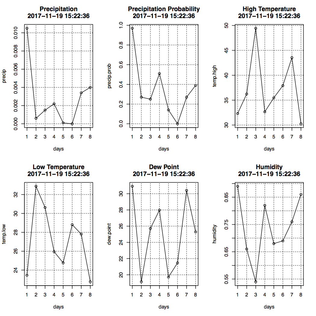
Figure 1. The First Part of the 8-Hour Forecast Plotted for the Indicated Date and Time.

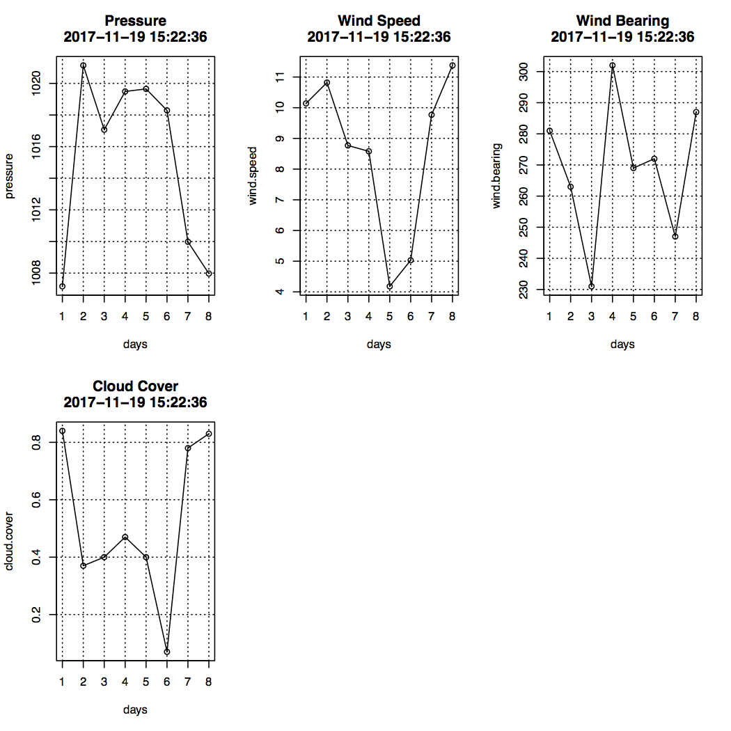
Figure 2. The Second Part of the 8-Hour Forecast Plotted for the Indicated Date and Time.

One could use the ‘precipitation’ forecast directly or have it multiplied by its probability, or perhaps have it augmented in some form or fashion by past weather. More on that in the next section.

2. Historic Weather

Of interest is potential precipitation. The historic data of rainfall extracted from the Deep Creek Hydro annual reports where they are part of the lake level data. The variables, lake level, rainfall rate, and cumulative rainfall are plotted for each of the years from 1994-2016 on a single graph, such as shown in Figure 3.

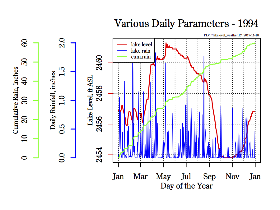
Figure 3. Lake level, Rainfall Rate, and Cumulative Rainfall for 1994.

All figures, in pdf format, can be downloaded from the following links.

It may be observed from the above set of graphs that the cumulative distribution is roughly the same from year to year.

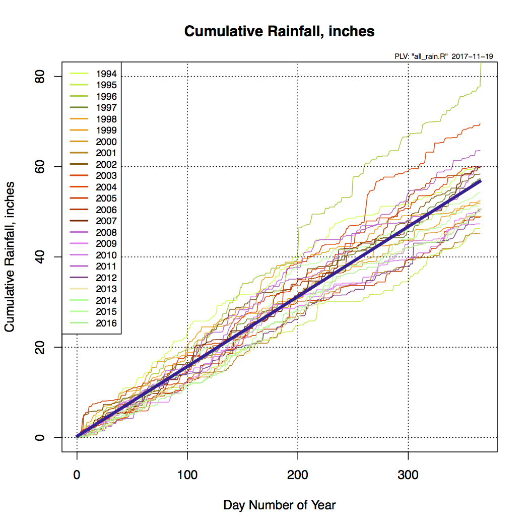
Figure 4. The Cumulative Rain Distributions for all Years, 1994-2016.

A straight line through roughly the center of the distributions is also shown. Such a line can be used to estimate the amount of rain that one could expect on given days.

Knowing the longest drought period, might be useful in developing a control strategy for maintaining a lake level such that needs can be satisfied without going to the lower rule band. It’s interesting to note the three spikes. These are quite extended time periods.

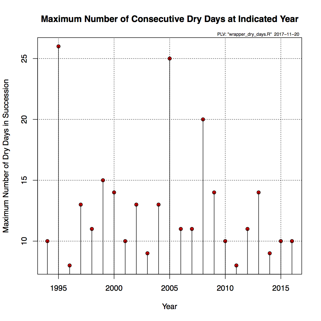
Figure 5. The Maximum Number of Consecutive Dry Days for 1994-2016.

The next level to look into is the number of shorter sequences, namely 5-day and 7-day sequences. These are more prevalent, as shown in Figure 5. One could almost detect a oscillating behavior on the 5-day sequence events, with a period of about 6 years. Such a number could be used to estimate the required the yearly lake reserve above the lower rule band.

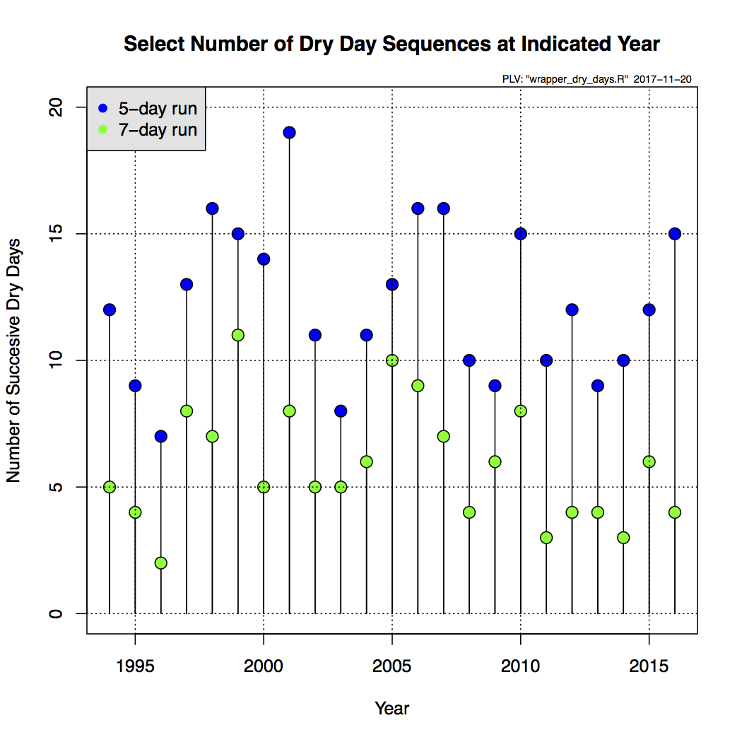
Figure 6. Number of Five and Seven Consecutive Dry Days Sequences for 1994-2016.

The probabilities of these events, can be determined by plotting the distribution for the whole year. A typical distribution is shown in Figure 7.

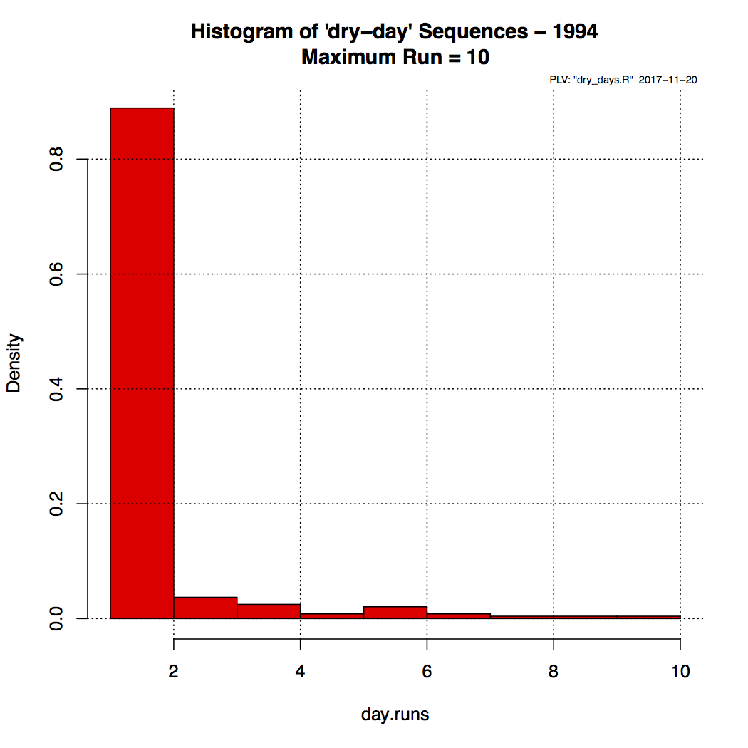
Figure 7. Typical Distribution of Dry-Day Sequences. Here for 1994.

Note that this seems to follow the 80-20 rule, where 80% of the occurrences are for 20% of the short duration dry-day runs. This is also known as the Pareto distribution. To understand just a little bit about the Pareto distribution check this video, named after Vilfredo Pareto (1848-1923), an Italian economist. This distribution is called a heavy tailed distribution, used to model extreme events. In insurance applications, heavy-tailed distributions are essential tools for modeling extreme loss, especially for the more risky types of insurance such as medical malpractice insurance. In financial applications, they provide information about the potential for financial fiasco or financial ruin. here, we could consider this for determining the maximum number of consecutive drought days.

The following are graphs of the drought-day-runs for all of the years for which we have data, 1994-2016.

PLV
First Published: 11/20/2017
Adapted for this website: 11/20/2017

Recent Titles

Categories

Weather Forecasts

1. Introduction

2. Historic Weather

Recent Titles

Categories

Tags

Weather Forecasts

1. Introduction

2. Historic Weather