Piet's Notes on Deep Creek Lake Science
Sensible Technologies - The Science of Deep Creek Lake
The concept of a ‘water budget’ was started by Morgan France during the development of the Deep Creek Watershed Management Plan in 2012. At that time the State had no interest in pursuing the idea. The Deep Creek Watershed Foundation, Inc. has subsequently pursued its development. This note attempts to express and extend Morgan’s thought processes in the form of a model and examine it against historical information published in Brookfield’s annual reports.
Since the development of the Deep Creek Watershed Management Plan, Morgan France (MF), one of the members of a subcommittee on water levels that was part of the development of the management plan, has been advocating the development of a ‘water budget’ model for allocating the waters of Deep Creek Lake equitably among its stakeholders. MDE and DNR have declined to develop such a model. There has been considerable confusion as to how to go about its development and what it would entail. After many discussions with Morgan, this note attempts to express his thought processes in the form of a model and examine it against historical information published in Brookfield’s annual reports. The basic conclusions is that it is possible to construct such a model. This report describes how I’ve gone about methods to develop such a model and tested it successfully against the lake level and generator status data for the years 2011-2016.
After many iterations with Morgan France, especially during the last few weeks (March 2017), I got his blessing that I understand his approach. And I must say, it actually makes sense in some ways. It is not a water budget in the traditional sense as one reads the literature and as I was mulling it over in my head and googling for approaches, but it could be construed as a water budget. However, I’ve taken a slightly different approach to implementing it than Morgan has with his Excel spreadsheets, but the result is essentially the same. The small differences depend on assumptions we both made.
In this note I explain the theory, the process as it applies to Deep Creek Lake, the implementation of a version of it with the computer language “R” [1, 2][the numbers in square brackets refer to references at the end of this report], and analyses performed against six years of historical data.
The results seem reasonable, but they also expose a number of ‘political’ and scientific issues that need to be dealt with to make this a tool for daily use.
This note only deals with the scientific issues, leaving the possible political aspects/ramifications to a separate discussion.
For the record, my previous reports about water budgets can be found here [3, 4].
On this web page I describe how I went about processing the available information.
The implementation process, to be described below, is based on the following assumptions:
1. At the time the calculations are performed it was assumed that we have no knowledge of future rainfall or the amount of groundwater entering into the lake. These two assumptions are automatically corrected when we do the next analysis the next day, but it does not allow for forecasting into the future. If, during the next day, it rains let it rain and groundwater recharge takes place until things dry up. Hence, the lapse of time between the two analysis automatically adjusts the lake level by additional groundwater flows and any possible rain and its impact on groundwater flows.
2. There is a time-volume release schedule for white-water rafting that is specified in the Water Appropriations Permit, the mandatory releases. This schedule also contains curtailment criteria should the water budget be unable to satisfy all demands. A few are specified in the Permit, such as when the lower rule band can or cannot be violated.
3. There is a TER (Temperature Enhancement Release) protocol for the conditions specified in the Permit. These depend on river temperature forecasts at the Sang Run river bridge. For water budget analyses, this could be made to be some statistical schedule based on past experiences. This may be a combination of modeling, let’s say for the next 10 days, to which is added statistical information for the remainder of the three months for which the TER is supposed to be evaluated according to the permit. There are several options available for a predictive capability which will be discussed later in the paper.
4. Modeling is only needed from April 15 to October 15. [7]
The ‘water budget’ model can be defined by the following steps:
1. Obtain the current lake level reading from the existing gage. (NOTE: There really should be a redundant gage at another location!)
2. Compute the available volume of water based on the current value of the lower rule band. The current volume is based on the stage-storage relationship previously defined as a result of bathymetric work performed in 2012. See another of my reports [xx]
3. Compute the daily water needs based on the white-water schedule defined in the Permit.
4. Estimate the amount of evaporation and remove it from the available water volume. This can only be grossly estimated based on existing data for the Savage Reservoir, although, with a little effort, a more accurate relationship can be developed for the lake.
5. Estimate the number of TERs that may be required. This can be done in a simple manner, using long range forecasts or statistically based on historic data. This results in some pseudo mandatory releases.
6. If there is still volume available, then Brookfield is allowed to generate power, with whatever schedule is dictated by their PJM contract or their own internal procedures.
7. The algorithm should be revisited every day. This would automatically incorporate any water coming into the lake via rain and/or groundwater.
As described above, the main forecasting model requires the following sub-models:
1. A revised TER protocol, because its error rate is too large, or perhaps done away with entirely.
2. A white water release protocol. Already spelled in the Permit, but may require tuning.
3. A water evaporation model. Not expected to be a significant contributor, but could impact allocations during hot and dry seasons.
These latter three items will not be addressed in this note
The following discusses the implementation of the water budget model as described above. It should be noted that the permit conditions involve a number mandatory time periods during which certain conditions have to be met. These periods are:
1. Totals for the year.
2. Daily amounts.
3. June, July and August.
4. June, July, August and September.
5. June, August and October.
6. Between April 15 and October 15.
To see how things work out with the proposed approach I will discuss the analysis methodology with past results. Specifically the model will be developed with data from 2012 and tested with data from 2011 and 2013-2016.
First, let’s see what the lake levels were during 2012 and how they related to the existing rule bands.
The daily average lake levels were obtained from the deepcreekscience.com website, a site that I created to collect all kinds of verifiable information about Deep Creek Lake. That data in turn was extracted mostly from Deep Creek Hydroelectric annual reports.
The first few lines of the 2012 lake level data file are shown below in Figure 1:
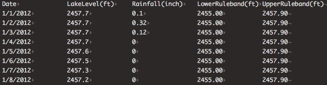
Figure 1. The First Part of the 2012 Daily Average Lake Levels.
The columns indicate the day of the year, average daily lake-level (ft AMSL - Above Mean Sea Level), daily rainfall (inches), lower rule band value (ft AMSL) and upper rule band value (ft AMSL).
The daily levels and rule bands are plotted in Figure 2. The rule bands were obtained from the latest version of the Permit [7].This is probably the worst year for hugging and even going below the lower rule band. It’s not clear what could have been done since we don’t have the history of the operation of the turbines, but from Figure 3, which shows the rainfall for that year, the year was not particularly dry or wet. However, given the number of TERs and bypass flow releases, to be shown later, the year must have been dry. While this information is not used in the methodology, it is of interest to see historically what is going on.
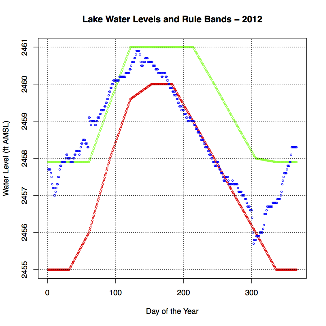
Figure 2. Daily Average Lake Levels for 2012.
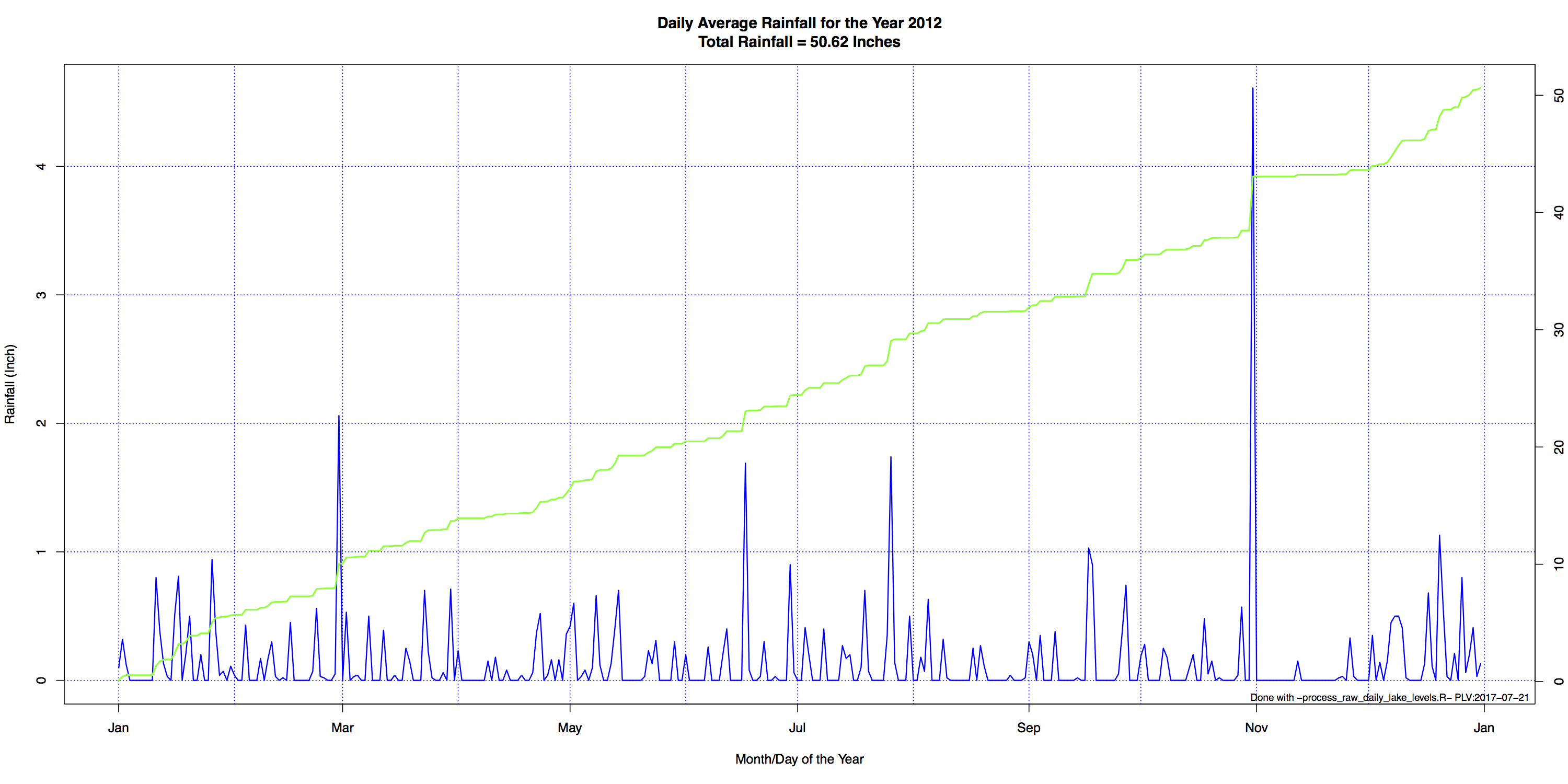
Figure 3. Daily Rainfall for 2012.
The next step is to develop the various mandatory release schedules. The white-water release schedule is specified in the Permit. It’s in terms of when and how long. The Permit data has been converted into a file that can easily be processed. Below, in Figure 4, are the first few lines of the white-water release file:
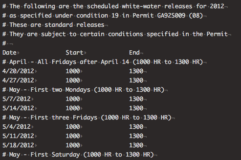
Figure 4. The first Few Lines Of the 2012 White Water Mandatory Release Schedule.
The next data file to be used is the TER release file. It’s easy to use past data since we have the actual release dates and durations. For a predictive model a combination of forecast TERs and statistical information is probably the way to go. Here, in Figure 5, are the first few lines of the historical TER data file for 2012:
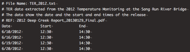
Figure 5. The First Few Lines Of the 2012 TER Releases as They Occurred.
There is one other mandatory data file to be derived from the annual report. This is the bypass data file. This information is also variable, because it depends on the flow conditions in the Youghiogheny river. The historical data as reported in the annual report are, as with the TERs, actual occurrences. In a predictive model the current day’s reading is clearly available, but future demands must rely on some kind of combination of forecasting and statistical data.
As quoted from the 2011 annual report “…when flows in the Youghiogheny River were less than 26 cfs. Flow data were obtained from the U.S. Geological Survey (USGS) recording at the Oakland gage, direct readings from the Oakland gage, or from the tailrace gage at the Deep Creek Station, per guidance provided in the protocol. Valve openings (see Appendix C) were determined from Table 3 of the protocol and were based on station operating status.”
It is not clear that the bypass setting is adjusted daily, but it is assumed to be such in the present analysis. Here, in Figure 6, are the first few lines of the 2012 bypass file:
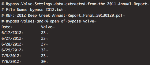
Figure 6. The First Few Lines Of the 2012 Bypass Valve Settings as They Occurred.
What is shown is the date and the valve setting. The setting is a function of the amount of flow at the Oakland USGS flow gage.
The valve setting has been correlated with the amount of flow that is bypassed using data from several annual reports and is discussed in one of my notes [5]. Figure 7 shows the results extracted from these reports.
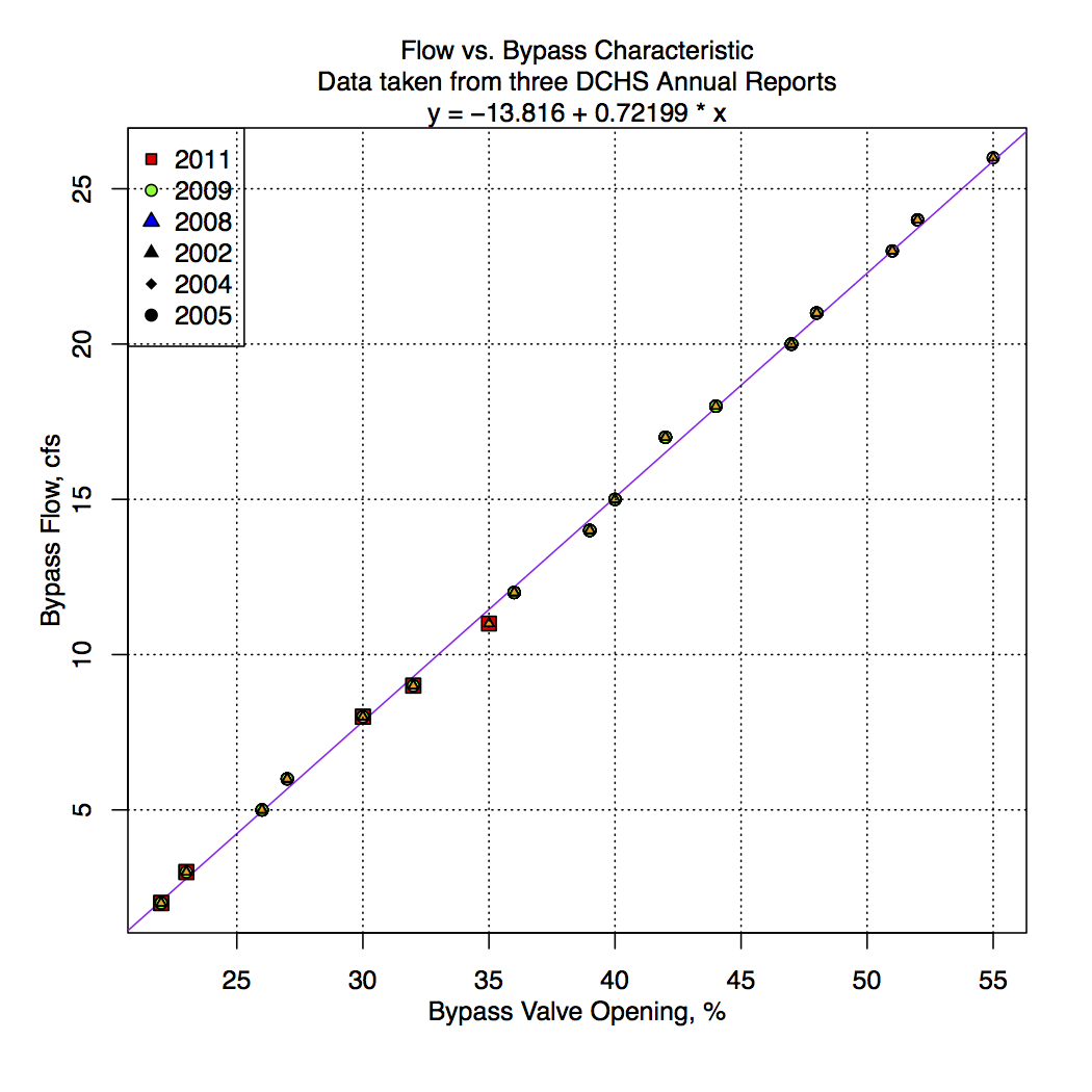
Figure 7. Daily Average Lake Levels for 2012.
The data from these reports have be fitted to a simple linear equation, giving the flow as a function of valve setting as shown in Figure 8:
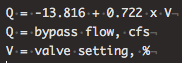
Figure 8. The Bypass Flow Equation.
The one remaining mandatory release is the 9 cfs through the wicket gates. This is a constant flow year-around, because this is wicket gates leakage, a flow that can only be stopped with expensive repairs to the turbines.
For now evaporation from the lake surface will be ignored.
All of these mandatory flow releases are now cast into a consistent set of total mandated daily demands. The unit of flow that will be used in the following discussions is acre-feet/day. Note that one acre-foot = 43,560 cubic feet.
One last item must be defined: the amount (volume) of water available in the lake between a given lake level and the lower rule band.
In an analysis performed a number of years ago, while defining the bathymetry of the lake, the stage-volume relationship was also determined. I wrote a report on that analysis [6]. Since only the upper part, say the top 10ft to 15ft, are of interest, an equation has been fitted to the bathymetry derived data. The resulting curve is given in Figure 9, showing that the lake is not a cylinder.
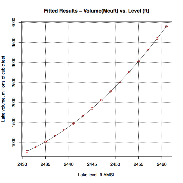
Figure 9. The Stage-Volume Diagram for the Upper 20ft of the Lake.
The resulting equation, obtained from a regression analysis using “R” functions, can be stated as shown in Figure 10:
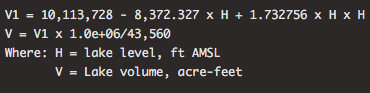
Figure 10. The Stage-Volume Relationship for the Upper 20ft of the Lake.
To find the available volume between a given lake level and the lower rule band one just evaluates the volumes at these two elevations, with the difference being the available lake water.
In the following graphs all y-axis values are cast in terms of acre-feet of water volume. This is because traditionally, in civil engineering circles, volumes of reservoirs have been stated in these terms because they are of sensible magnitudes. At the same time these quantities are easy to display on graphs.
Putting it all together one gets the results for the year 2012 described in the following set of figures.
First the white-water releases. Figure 11 shows the water volume required, in acre-feet, for the days specified in the Permit.
I’m sure that the peak is noted. This is specified in the permit for the “Annual Team Friendsville Upper Youth Race,” an extended 6-hour release. Normally the releases are for 3 hours.
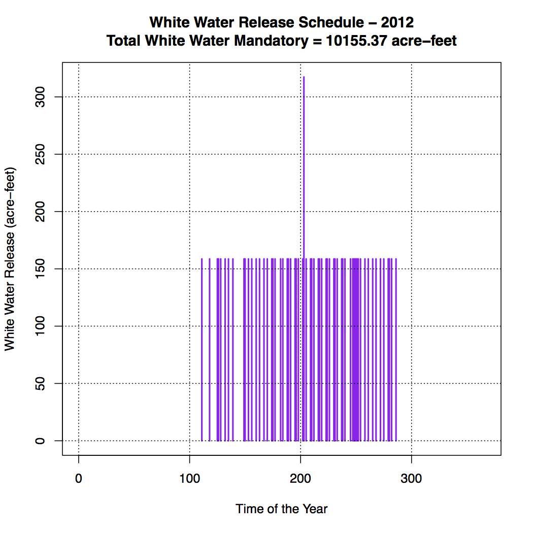
Figure 11. White Water Releases Made During 2012.
Figure 12 shows the water volumes associated with the TERs.
Figure 12. Water Releases Associated with TERs During 2012.
Figure 13 shows the bypass flow schedule. This is also mandated in the permit, and is a function of the Youghiogheny flow at Oakland. The Permit requires that a minimum flow of 40cfs must be maintained below the tailrace at all times. Furthermore, a reduction in the minimum flow below 40 cfs may be requested of the administration when the reservoir levels are one foot or more below the lower rule band.Hence it can vary.
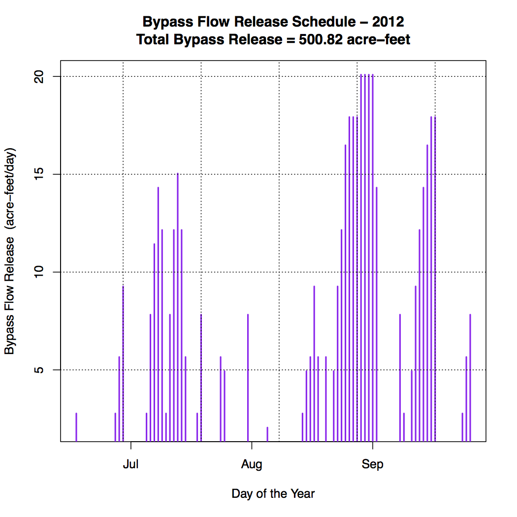
Figure 13. Bypass Flow Releases During 2012.
Figure 14 shows yet another required flow, namely leakage through the wicket gates. It is specified as a requirement in the Permit. However, I don’t believe that they (Brookfield) have much choice. This is ‘natural’ leakage because the wicket gates, which basically function to control the flow through the turbines, are wearing out and are very expensive to repair or replace.
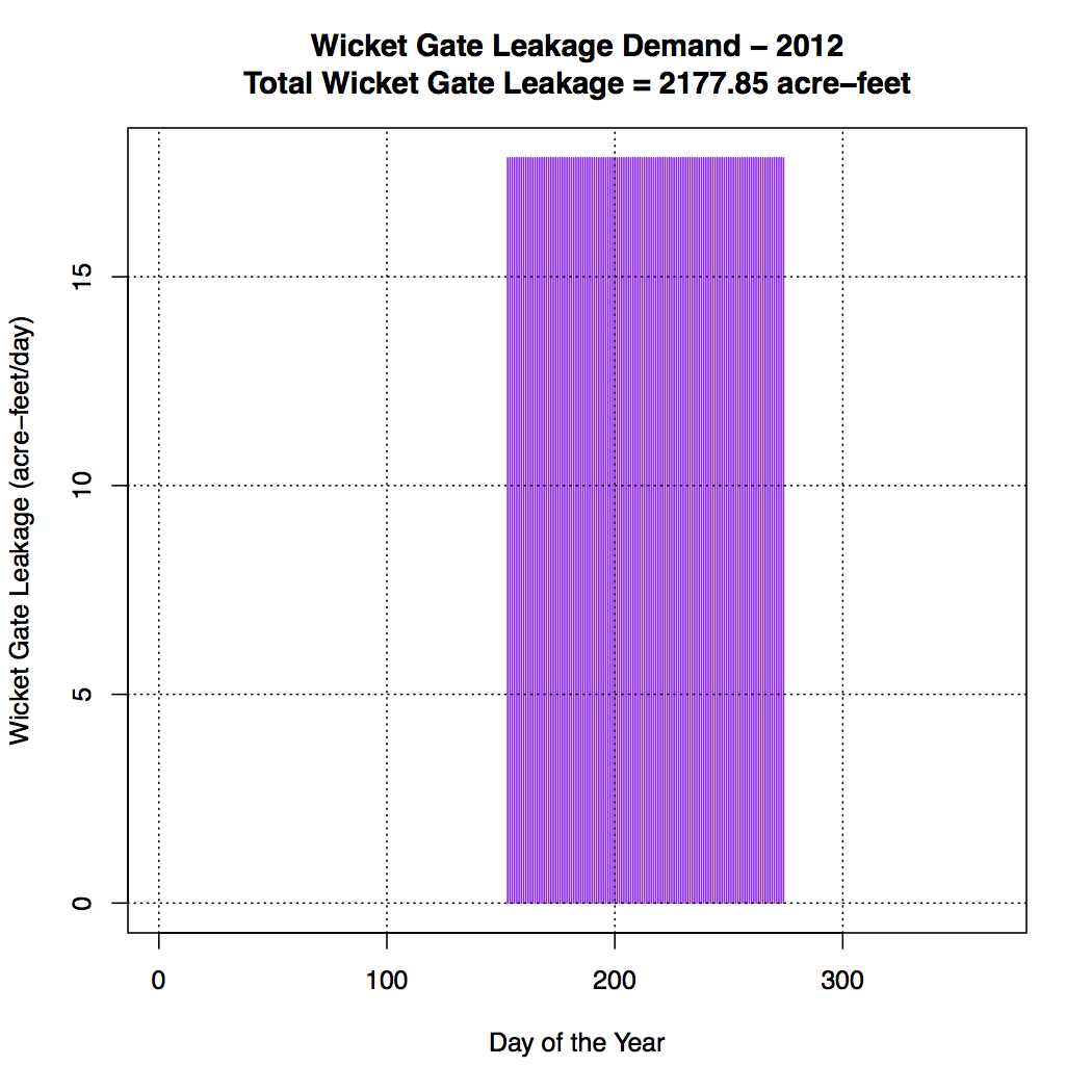
Figure 14. Wicket Gate Releases During the Period of Interest in 2012.
And the final result for all of the demands together is shown in Figure 15. This is basically the sum of Figures 11, 12, 13 and 14.
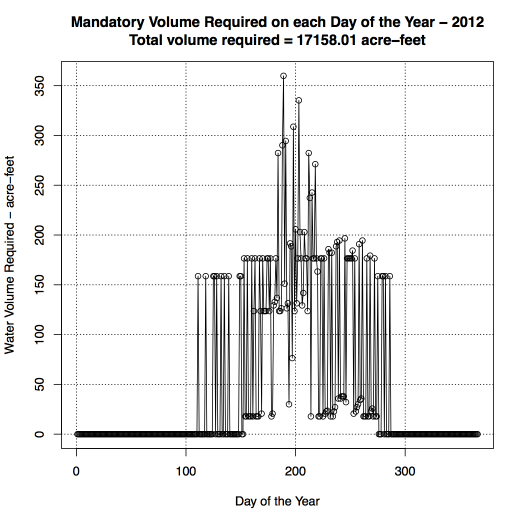
Figure 15. Mandatory Volume Flows Required During 2012.
The total daily water volume available is shown in Figure 16. These are the result of calculations whose methodology are described earlier in this paper.
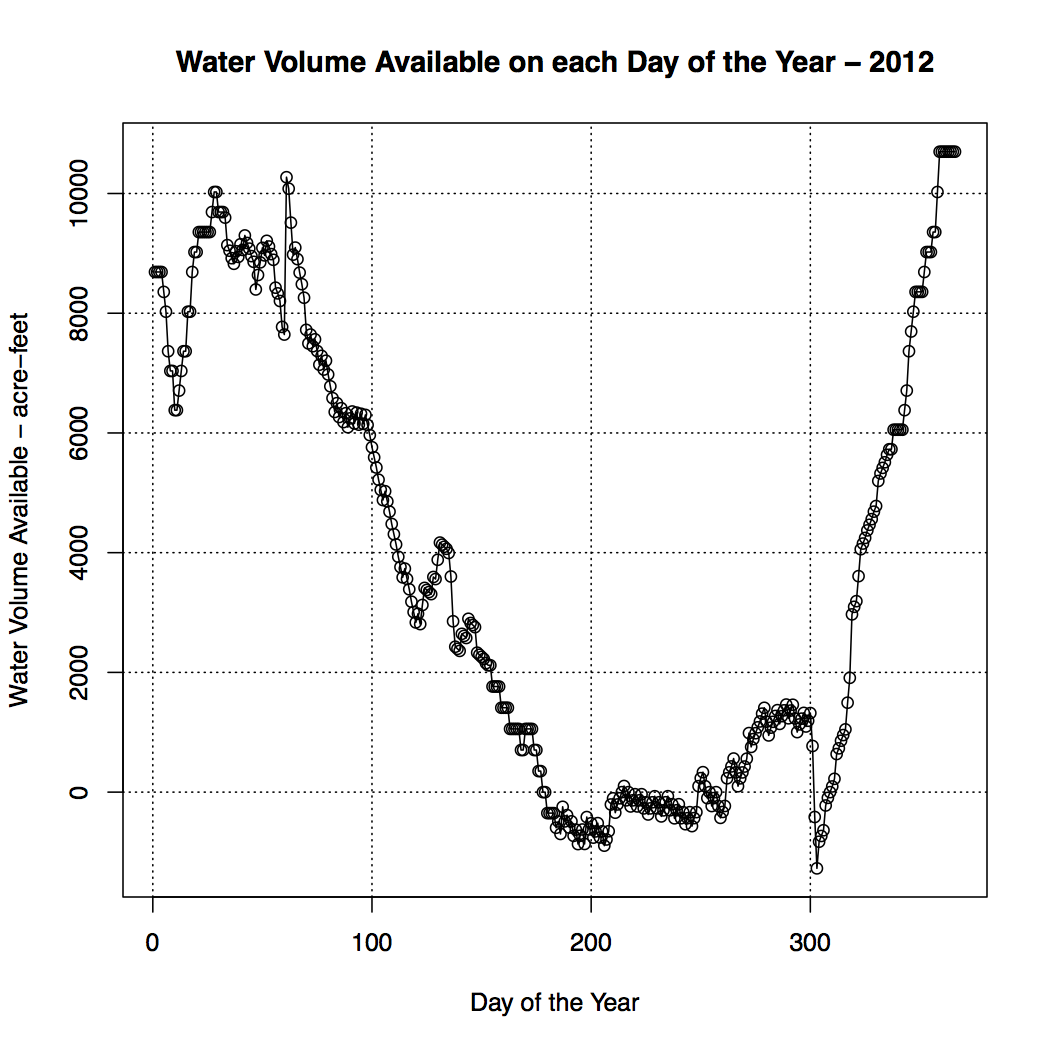
Figure 16. Water Volume Available During 2012.
The next graph, Figure 17, would normally show the difference between the daily available volume and the daily demand volume. However, the two curves look almost the same so both, available and demand have been plotted on the same graph and are shown as Figure 17. The green dots are the available volume numbers, while the red dots are the net remaining volumes, meaning daily available minus daily demand.
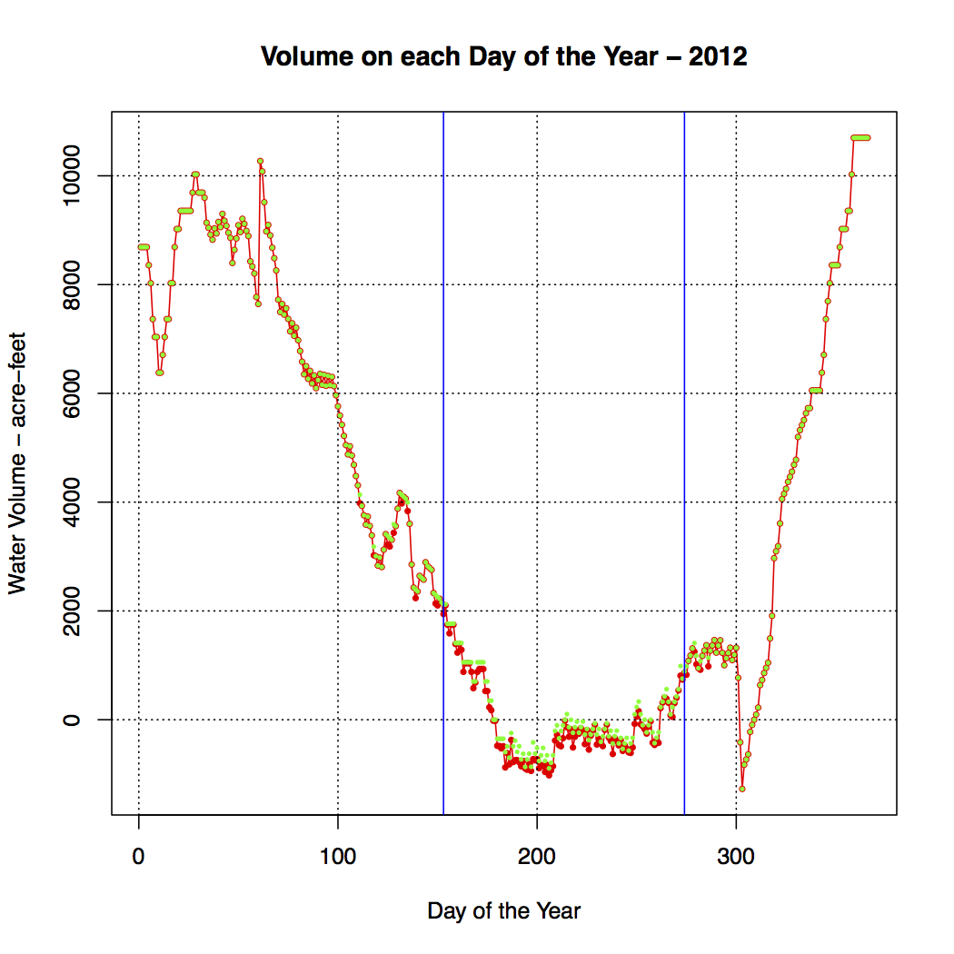
Figure 17. Water Volumes During 2012.
DO NOTE, the discretionary releases have not been taken into account. A discretionary release is a release elected by Brookfield to generate power. That will make the curves look different before the first and after the vertical blue lines in Figure 17 (day 152 and 273). In between these two lines there are no discretionary releases because plenty of power is made via the mandatory releases.
The reason the discretionary releases have not been taken into account is because they are not available from the literature. They could possibly be reconstructed from the USGS river flow gage data but this has not been done. They are not going to change the basic issues that exist during the Permit period, from day 152 to day 273, April 15 through September 15.
The analysis described above has been performed for the years 2011-2016. The relevant results and input data are given below
The outputs from the analyses:
1. Analysis results for 2011
2. Analysis results for 2012
3. Analysis results for 2013
4. Analysis results for 2014
5. Analysis results for 2015
6. Analysis results for 2016
The daily average lake levels:
1. Daily average lake levels for 2011
2. Daily average lake levels for 2012
3. Daily average lake levels for 2013
4. Daily average lake levels for 2014
5. Daily average lake levels for 2015
6. Daily average lake levels for 2016
The bypass settings and release dates:
1. Bypass settings for 2011
2. Bypass settings for 2012
3. Bypass settings for 2013
4. Bypass settings for 2014
5. Bypass settings for 2015
6. Bypass settings for 2016
The TER release dates:
1. The TER releases for 2011
2. The TER releases for 2012
3. The TER releases for 2013
4. The TER releases for 2014
5. The TER releases for 2015
6. The TER releases for 2016
The white-water release dates:
1. The white-water releases for 2011
2. The white-water releases for 2012
3. The white-water releases for 2013
4. The white-water releases for 2014
5. The white-water releases for 2015
6. The white-water releases for 2016
All of the calculations were performed with “R”. All software and data has been assembled in a zip file which can be downloaded here.(forthcoming, perhaps)
1. Ashley Vance, R You Ready for R?, The New York Times, January 8, 2009 Paul Krill, Why R? The pros and cons of the R language, June 30, 2015
2. The Foundation’s ‘Water Budget’ Research Program P. Versteegen, DCL217, June 6, 2016
3. Constructing a Water Budget for Deep Creek Lake, A Definition of the Problem P. Versteegen, DCL013, May 5, 2014
4. Turbine Bypass Flow P. Versteegen, DCL074, March 6, 2014
5. Stage-Storage Diagram P. Versteegen, DCL161, August 30, 2013
6. Deep Creek Lake Permit Versions BROOKFIELD POWER PINEY & DEEP CREEK LLC - GA1992S009(08), MDE
PLV
First Published: 4/2/2017
Revised: 8/9/2017
Reformatted: 11/14/2017