Piet's Notes on Deep Creek Lake Science
Sensible Technologies - The Science of Deep Creek Lake
The TER is an elusive issue. One the one hand logic says that it would help brown trout to be happier in the Youghiogheny River between the tail-race and the Sang Run River bridge, on the other hand releasing water using an algorithm that cannot be shown to do its job would seem to imply that we don’t need an algorithm. Just release water periodically will keep everyone happy.
I like to explore these thoughts here and show the latter option is probably the easiest and most reliable way to go about it.
So, I ask myself the following questions:
1. Where is the evidence that TERs definitely work?
2. Where is the evidence that, in that stretch of the river, the Yough is a popular fishing region?
Much of my thinking comes from reading the 1994 Penelec report in support of their application to the State of Maryland for a water use permit, and a recent Spanish paper that purports that daily average water temperatures are a far better gage for measuring fish well-being.
Note that everyone should read the 1994 Penelec report. It provides a great narrative of the state of affairs around and in Deep Creek Lake in the early nineties and the underlying philosophy of the current permit.
The first question to ask is: Do TERs work?
The 1994 Penelec report describes in detail the experiences of Penelec over the years with managing not just the lake, but also the fisheries and white-water rafting of the Youghiogheny River. This is a natural consequence of Penelec wanting to do as much power generation as possible.
A number of statements are made in the Penelec report that are important to the river temperature issue.
But before we get started with this, it should be noted that the stream is a mountain stream meaning it has some very specific characteristics different from rivers and creeks that flow in flat lands. First it follows valleys that have a significant gradient, causing water to flow relatively rapidly. Secondly, that characteristic carries away all of the small particles, leaving often a rocky or rock-strewn bottom/river bed.
One can understand that a constant release would definitely benefit the trout population. But is this natural? While Deep Creek Lake impounds the water from Deep Creek and other streams, all of that water eventually winds up in the Youghiogheny. If there were a drought, Deep Creek and other tributaries feeding the lake are, most likely, also low flowing and subjected to heating by sun and ambient temperature. Hence in the “pre-lake” times river temperatures would get hot and, to survive, fish would have find their preferred hiding places. Looking at old maps, Deep Creek flowed through marshland and hence did not have a lot of shading. I’m sure that temperatures in those days would go above 25 °C a fair number of times.
A second point is that the Yough river bed is essentially rock (as per Penelec 1994). That means that there is an infinite heat sink/source reservoir of 55 °F (12.8 °C). Solar radiation is the essential cause of water heating at low flows when they are calm and hence clear, non turbulent flows. Radiation impinges on dark surfaces where it gets absorbed and causes the heating of rocky materials. The low flows may already be hot coming into the river segment of interest. The typical weather patterns are cycles of days with increasing temperatures followed by a day thunderstorms with a lot of water runoff and colder temperatures.
A recent paper found that day-average temperatures are a better predictor for the health of a fish habitat.
Given all of this, one could conclude that, rather than a 2-hr two turbine release, it would be far more beneficial to do a 4-hr one turbine release allowing time for the rocky river bed to cool down by the passage of cold water from the release, or probably even better, an 8-hr partial operation of one turbine, or perhaps a full-open bypass flow or a combination thereof.
All of this requires an analysis and comparisons with measured data.
The next question is: “Where is the evidence that the Yough is fished by many people?”
There is no real data, at least none that anyone is willing to share!
I have had casual conversations with people that raft and fish and with someone who has flown over that stretch of the river a number of times this summer, at least 8. The common answer seems to be that nobody is fishing!!! Even language in the Penelec 1994 report suggest that this section of the Yough is not necessarily good for trout because of the absence of “hiding” places. But, I’m sure that avid fisherman will contradict this. All I can say is: “Show me!”"
Furthermore access to this stretch is hampered because of the existence of a lot of private properties bordering the river and strict government regulations that prevent the construction of easy access path and areas. Difficult access is because “In 1976 a 21 mile long segment of the Youghiogheny was designated as Maryland’s first Wild River. A state protected corridor along the river runs from Miller’s Run just north of Oakland to the town of Friendsville. This corridor is managed by the Maryland Park Service to preserve the wild and natural scenic, geologic, historic, ecologic, recreational, fish, wildlife, and cultural resources.”
One could easily conclude that stocking fingerlings and TERs by the current protocol are a waste of time and money. Perhaps, as suggested above, a regular one-turbine 4-hr release every day, at around 1pm and staying above the lower-rule band, would probably accomplish more for the well-being of any fish.
To show that the above suggested operation is a better alternative for managing cold water one needs to look at the heat transfer effects happening in the river bed. With some simplifying assumptions this, in principle, is not a difficult problem to solve.
(10/8/2017) I started out by finding analytic solutions to various riverbed applicable problems and found this reference to be usable.
But, what a really wanted was a capability to change the boundary conditions, that is, the water temperature and incident heat flux, in a arbitrary manner. For that I need a numerical tool to do this.
I found in the literature some course notes on the derivation of the appropriate equations on this exact problem and a listing of the numerical solution in ‘matlab’ code. I was able to convert that code successfully to “R” code and am now able to run arbitrary problems.
Figure 1 shows code result comparisons of different numerical integration schemes against the results from an analytical solution, all of which were produced by the above matlab reference from which the source code was implemented. As one can see, the results agree very well, validating the implementation. Compare this with the results, shown in Figure 2, obtained from the referenced matlab source.
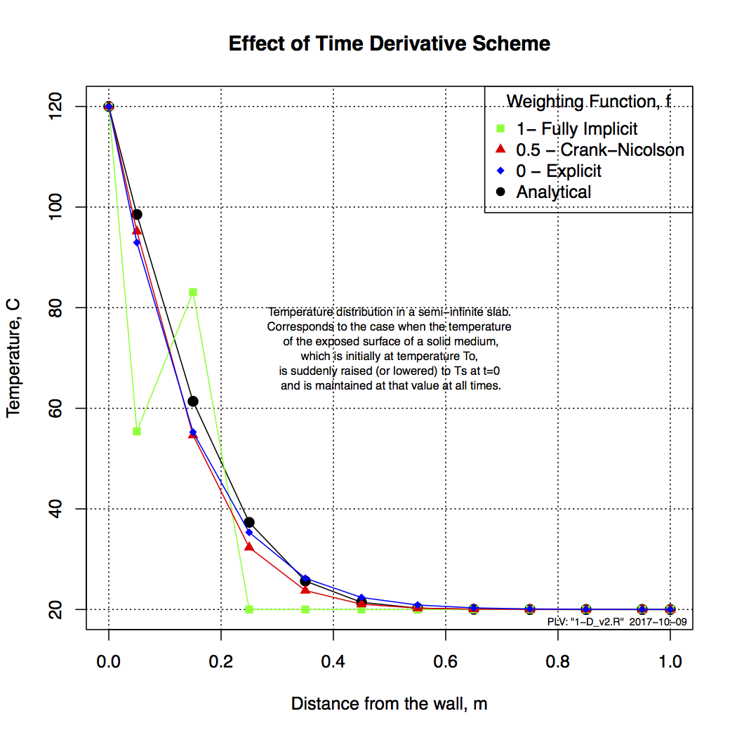
Figure 1. The Validation of the Implementation.
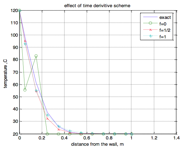
Figure 2. Reference Result from the Code Source.
Now that I have a tool to examine heat transfer effects between a rocky surface and flowing water we can try to examine to see how much heating and cooling occurs in a diurnal cycle.
But first one should look at which solution option to use in our analysis, explicit, semi-implicit, or fully implicit. The natural reaction would be the latter one, the fully implicit method.
Let’s check this out with a problem in which the surface of a rock slab, which is initially at 15C is suddenly exposed to a temperature of 50C for 1 hr and then suddenly put back to 20C.
To do this we need properties of rock, namely density, thermal conductivity, and heat capacity.
A Google search revealed the following data sources: The next step is to find appropriate rock properties, river temperature profiles, and solar radiation flux profiles, to examine the net heat fluxes occurring at the surface of the semi-infinite slab.
There are several references to properties of rock. Here is one. Rock properties, thermal conductivity, density, and specific heat respectively, have been extracted from this reference used are:
κ <- 1.0 # Thermal Conductivity. For most rocks, varies between 0.5 and 4.2 W/m/K; used 1.0
ρ <- 2500 # Density. Varies between 1500 and 3300 kg/m^3; used 2500
c~p <- 750 # Specific Heat. Varies between 500 and 1000 J/kg/K; used 750
Specifically for granite these numbers are: κ <- 2.5 # Thermal Conductivity, W/m/K
ρ <- <- 2670 # Density, kg/m^3
c~p <- 950 # Specific Heat, J/kg/K
But first, the code has been cleaned up and made solely into an implicit methodology. Furthermore, a routine has been added to define the surface temperature boundary condition at any time. Also, an ability has been added to plot select temperature profiles during the period of the solution.
An example of the result of this effort is shown in Figure 3 and 4. A uniform slab at ambient temperature was suddenly exposed to a constant surface temperature for 2,000 seconds and then held at ambient temperature until 3,000 seconds. The time step used was 1.5 seconds. The time of the profiles are indicated in the legend. Figure 3 uses ’typical’ rock properties, while Figure 4 is done with the thermal properties of granite.
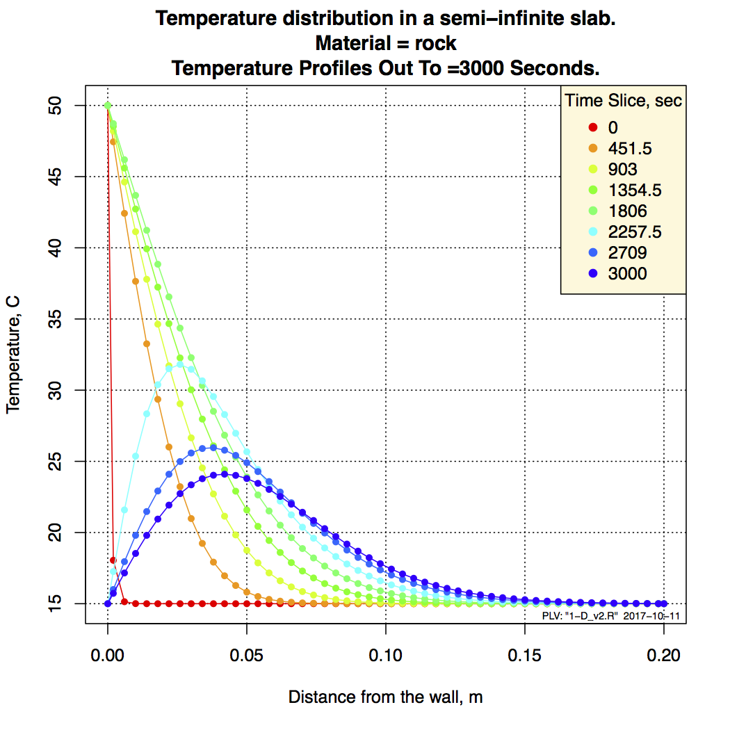
Figure 3. Sudden Temperature Exposure for a Finite Duration on Rock Surface.
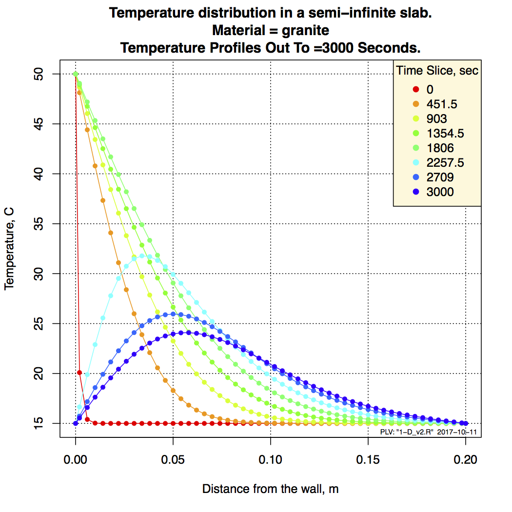
Figure 4. Sudden Temperature Exposure for a Finite Duration on Granite Surface.
The next step is to add a more complex boundary conditions, namely an impinging heat flux, to simulate solar radiation, a heat transfer loss from the surface to a fluid flowing past the surface to simulate a cold/warm stream flowing over the slab and a combination of the two.
(10/13/2017) This has now be done. The code has been modified to handle the following types of boundary conditions on the interface of the slab:
1. A specified temperature profile on the surface of the slab (bc=1). For a result see Figure 4.
2. A specified profile at the surface of a convective heat transfer process at the surface to a flowing medium (bc=2). See Figure 5 for an example result for a granite slab.
3. A specified heat flux at the surface (bc=3). See Figure 6 for an example result for a granite slab.
4. A combination of 2 and 3, s specified heat flux and a specified convective profile (bc=4). For an example result see Figure 7.
Solar radiation is easily specified. It goes from 0 to a max and back down to zero. The magnitude depends on the sun angle with respect to the surface. A maximum value of xx watt/m^2 will do for here.
The basic geometry of the problem that 1-D solves is described in Figure 5.
The surface is described by temperature node T1, which is much smaller in size than the next neighbor, T2. The node T0 is the flowing stream temperature. Convection takes place between the surface node and the stream node. The impinging heat flux, q”, is shown at the surface.
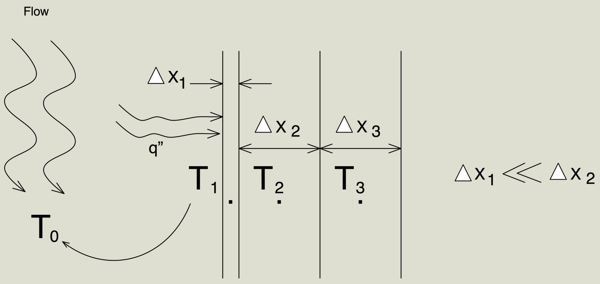
Figure 5. A schematic of the 1-D geometry and its temperature nodes.
The 1-D code was developed in terms of knowing the surface temperature T1 (bc=1). The other boundary conditions can be converted in terms of T1 by doing a simple energy balance at the surface. Thusly it can be easily shown that for a purely convective type of heat transfer at the surface (bc=2):

Figure 6. A schematic of the 1-D geometry and its temperature nodes.
For a pure heat flux impinging on the surface the relationship is (bc=3):
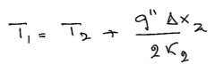
Figure 7. A schematic of the 1-D geometry and its temperature nodes.
And lastly, for a combination of convection and heat flux the relationship becomes (bc=4):
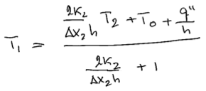
Figure 8. A schematic of the 1-D geometry and its temperature nodes.
In all cases, the stream temperature, convective heat transfer coefficient, incident heat flux, and fixed boundary temperature can all be specified as a function of time.
Example output for each of these cases are demonstrated in Figures 9, 10, 11 and 12. The behavior shown in the graphs is what one would expect.
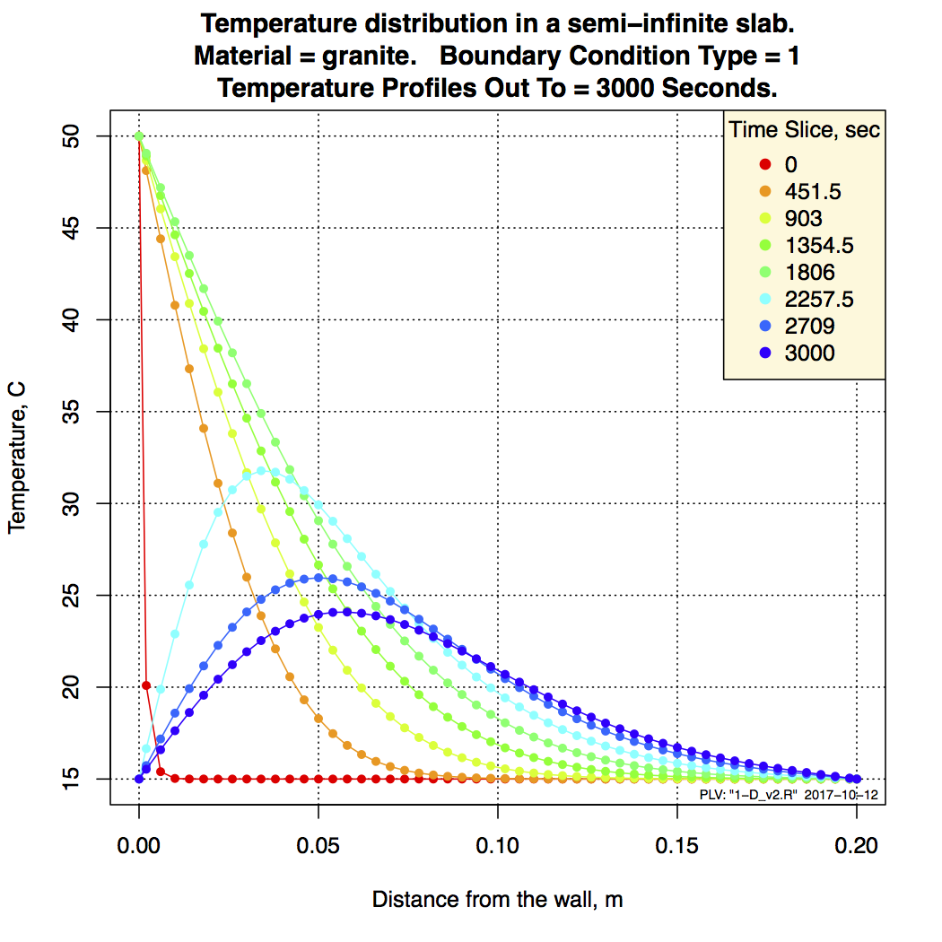
Figure 9. Temperature suddenly raised to 50 °C then dropped to ambient at 2,000 sec.
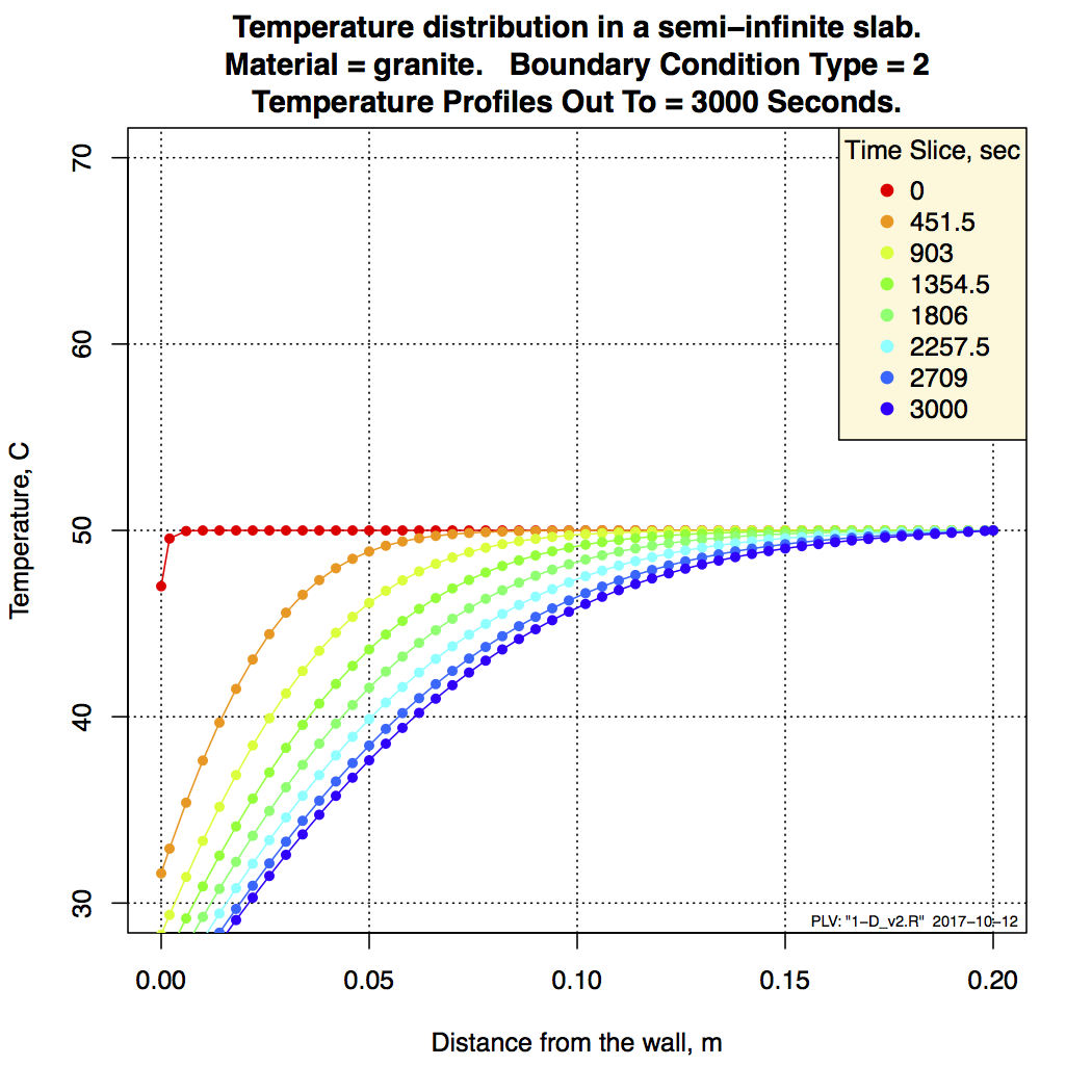
Figure 10. Intital slab temperature at 50 °C and stream at 15 °C with h=100 w/m^2-C.
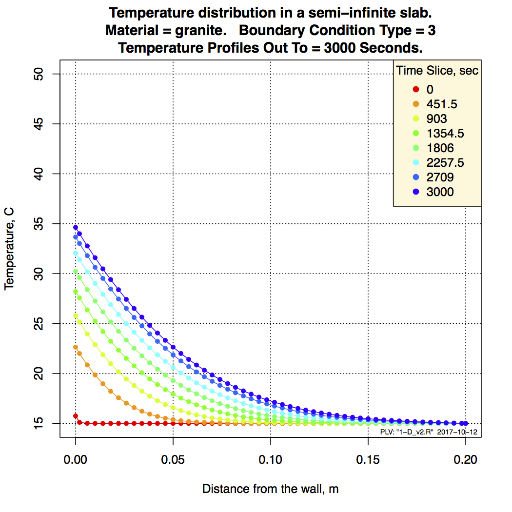
Figure 11. Slab at 15 °C with incident heat flux at 800 w/m^2.
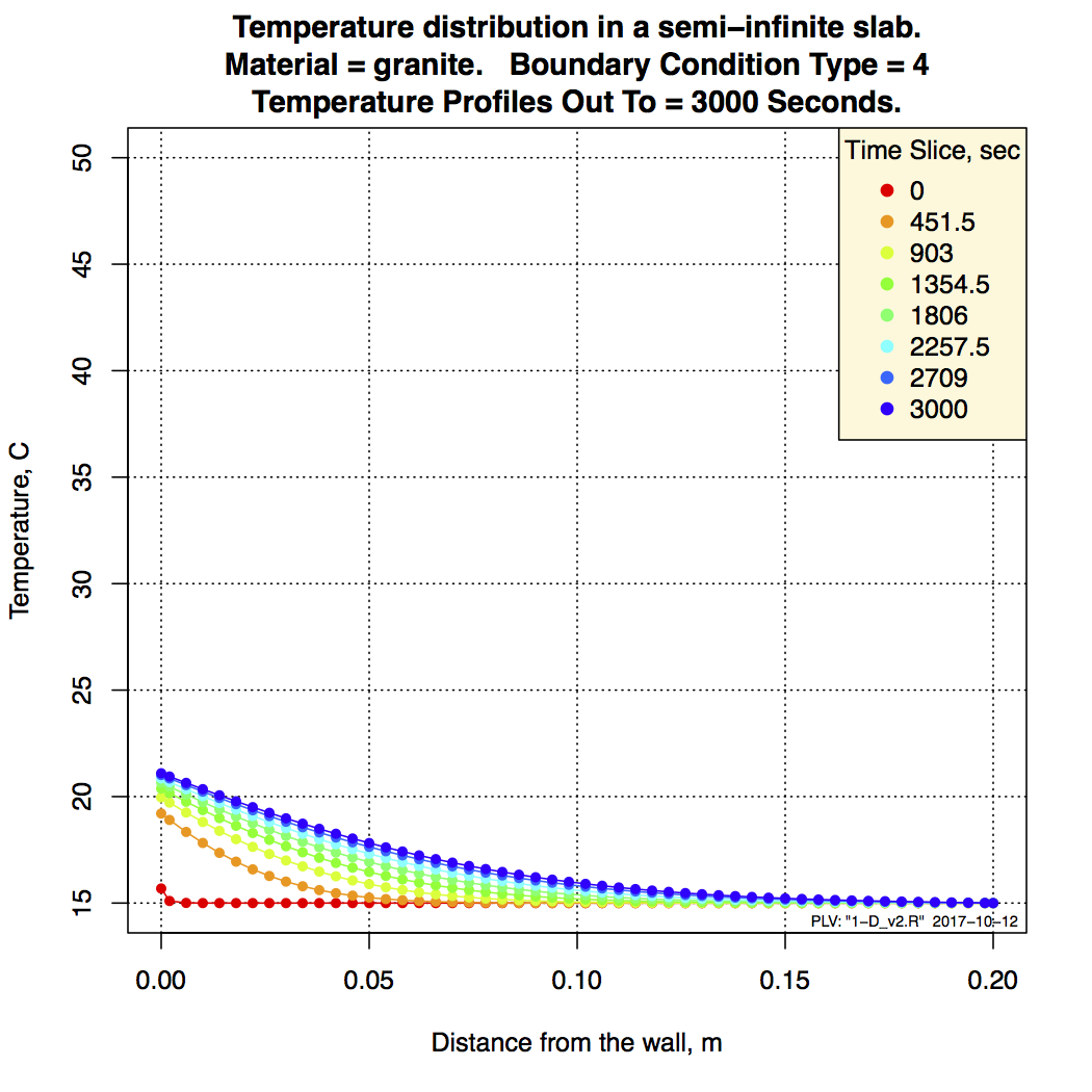
Figure 12. Conditions from Figures 7 and 8 simultaneously.
Onto something perhaps more realistic. (10/15/2017)
Much of the ground in Garrett County is compromised of sandstone. Sandstone is a complex rock material. Articles have been written about it, such as this one, from which its thermal properties have been extracted for our purposes.
The bulk density of selected sandstones studied in the above referenced article ranges between 1868 kg/m^3 and 2651 kg/m^3. Sandstone appears with different volumetric moisture content. Thermal conductivity ranges from 1.23 W/m/K to 5.68 W/m/K. Specific heat varied from 645.62 J/kg/K to 1298.3 J/kg/K. In other words, there is a wide range of values for each.
Middle of the range values have been chosen for this study, namely 2260 kg/m^3 for density, 3.46 W/m/K for thermal conductivity, and 972 J/kg/K for specific heat.
These are not quite the same as those given in another important material property reference (see here), but that’s what we’ll use for now.
Plugging these properties into the current code gives the results shown in Figure 13.
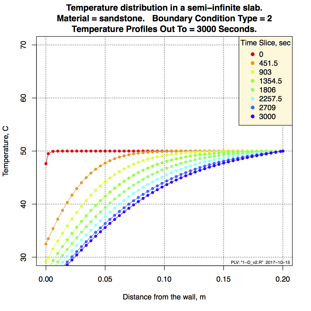
Figure 13. Initial slab temperature at 50 °C and stream at 15 °C with h=100 w/m^2-C.
Compare these results with those of Figure 7. One can see a deeper penetration of the thermal front in the sandstone than in the granite (look at the location of the 3,000 sec curve). Does this make a difference?
What we really need to do is to couple this with a control volume of water and investigate how the temperature of that volume of water changes when subjected to various values of boundary condition type 4, heat flux and convection.
PLV
First Published: 10/1/2017
Revised: 10/15/2017
NOTE: The script that replicated the validation problem can be found here.
The script that produces Figures 3, 4, 6, 7, 8, and 9 can be found here.