Piet's Notes on Deep Creek Lake Science
Sensible Technologies - The Science of Deep Creek Lake
In 1994, The Pennsylvania Electric Company (Penelec), owner and operator of the Deep Creek Hydroelectric Station, obtained from the Maryland Department of Natural Resources (MDNR) Water Resources Administration (WRA) a ‘Water Appropriations Permit’ to operate the Deep Creek Hydroelectric Station for power generation.
Condition 16 of this permit required Penelec to submit a plan for operating the project to maintain temperatures of less than 25 ℃ in the Youghiogheny River between the Deep Creek HydroElectric tailrace and Sang Run, 5.8 km (3.6 miles) downstream (Figure 1). The purpose of this condition is to enhance cool-water habitat for trout in this reach of the river. In the plan, temperature was designated as the primary factor determining fish habitat quality; thus, improving the conditions for the fish by lowering the water temperature to a suitable range is incorporated in the term “temperature enhancement.
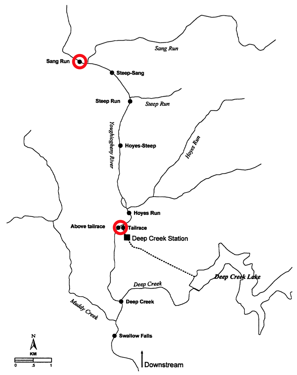
Figure 1 - Map of the Youghiogheny River between Swallow Falls and Sang Run showing the locations of Deep Creek Station tailrace, temperature sampling stations and major tributaries.
Penelec outlined a general temperature enhancement protocol (Penelec 1994 for operating the power plant to:
The name of the release is a bit of a misnomer, since the release does not enhance (aka increase) the temperature of the water of the Youghiogheny river, but rather it attempts to cool its waters down to 25C or below, at the Sang Run bridge. Apparently the term “enhance” is to reflect the enhanced habitat conditions for the brown trout.
The goal of this development effort is to have an accurate and simple to use computer model for predicting the water temperature on an hourly basis at the Sang Run bridge of the Youghiogheny river in order to determine whether a release through the generators should be executed.
To develop a river temperature model that can provide a 24-hour temperature forecasts at the Sang Run bridge accounting for arbitrary water releases coming from the tail race of the Deep Creek Hydroelectric project and a protocol to determine the required length of a release to maintain the temperature at Sang Run bridge under 25 ℃.
The eventual outcome of the objective is visualized to be a software product that runs automatically every day during the summer period and provides a suggested list of operations and timing for Brookfield’s Deep Creek Lake Hydroelectric generation facility, the power-plant.
It is visualized that it will provide an accurate 24-hr forecast as to when and for how long the power-plant should operate at full power to make sure that the temperature at the Sang Run bridge remains 25 ℃ or below. Such a forecast would allow the white water rafting companies to alert their clientele as to the availability of good rafting waters. Such schedules would be posted on Brookfield’s website.
For it to be a fully automated system will require certain initialization and weather forecast data that have to be retrieved from remote locations. Provisions should be made in case such data cannot be collected for whatever reason. The development of the methodology may specify some specific data to collect, but all efforts will focus on using information that exists already.
So how could this work?
Computer systems can be programmed to start a task at regular times. For now we shall assume that daily run is required. It may be possible that longer forecasts can be made. This may be possible when there is no rain in the forecast.So assume that a forecast is generated every noon of every day. The process is started by automatically collecting meteorological and river flow and temperature data.
NOTE: There currently is no flow and temperature gages upstream of the tail-race, nor is there meteorological data. It is strongly recommended that a flow and temperature gage be installed in the river and that a conventional meteorological data acquisition system be place near that location. The data station should provide the following parameters:
•	Air temperature
•	Wind-speed
•	Direct solar radiation
•	Total insolation
•	Relative humidity
•	Barometric pressure
•	Precipitation
•	River water flow-rate
•	River water temperature
The data should be collected at 5 minute intervals (this time span is in sync with the way the lake water levels are recorded). The operation of this station should be checked constantly to assure its proper operation. ]
The collected data should be run through some kind of validation process to ensure that the numbers are valid. The data could be checked against some collected earlier or the previous data; it should be check that it is in the range of averages expected, etc. Details to be worked out.
In case the collection station is down, extrapolations from a previous set, or invented data based on historic data, or similar profiles, to be defined, should allow the forecasting process to continue.
The idea here is to define what it is that one wants the model to do. Once one understands that, then one can define the specific computational procedures and data structures that are needed.
The goal and objective is to compute the water temperature at one point in the Youghiogheny river. to compute forecasted temperatures over a stretch of the river. The temperature range likely to be involved in is from around 10 ℃ to 40 ℃. Since we need to look at whether 25 ℃ is exceeded or not, the temperature range is pretty small, and the uncertainty should probably be within 0.5 ℃.
When one compares predictions against experiments, the measurement has to be something that the model can predict.
First of all we need to account for all of the energy terms that are likely to play a role. A detailed review of the literature should reveal all the terms that should be accounted for. A lot of literature has already been read or scanned, and Ref. 1 stands out as good starting point. From this paper, the following energy energy terms appear to be appropriate. Solar radiation (direct, indirect, and diffuse)
One of the crucial debating points in developing the Deep Creek Lake Watershed Management Plan is whether the releases from the lake are overkill. It is suggested that the bypass flow could be used to control the river water temperature.
Based on simple caloric arguments this appears to be possible, but many have expressed doubts using this argument, because the water, over its travel time to the location where temperature is measured, will be exposed to all kinds of positive and negative heat transfer processes.
This part of this web page has taken equations derived for predicting various aspects of river water temperature changes and programmed them for a unit distance and performed sensitivity studies indicating whether the simple caloric balance argument would provide incorrect results.
As with the water budget for the lake itself, there is a conservation of energy relationship (energy budget) that dictates how water temperature changes:
change in heat storage = net heat flux = heat energy in - heat energy out
The basis for the results to be described in this note are Equations (11) through (37) and the constants of Table 1 of reference 1.
From various references one sees figures depicting the mechanisms that are in operation when water flows through a river bed. Figures 2-6 are such figures. They all depict the same kind of thing, but in different ways and with different detail.
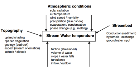
Figure 2. Factors Influencing Thermal Regime [1].
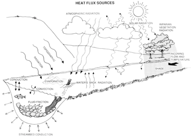
Figure 3. Schematic of Energy Components that Affect Water Temperature [2]
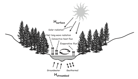
Figure 4. Scheme of energy fluxes that influence temperature of mountain streams [3]
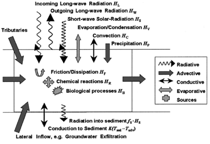
Figure 5. Scheme of energy fluxes that influence temperature of mountain streams [3]
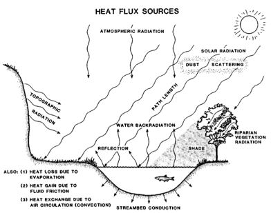
Figure 6. Scheme of energy fluxes that influence temperature of mountain streams [8]
It’s typical to consider the following factors:
The approach used here is to take a control volume through which water flows from one end to the other. There is an option to introduce water on the side at a specified flow rate and temperature.
The river is assumed to be 50 ft wide and 3 ft deep. The basic length of the control volume is chosen to be 50 ft but can be changed.
The method requires a lot of data. For the present purpose, the following values are the basis from which all calculations are performed unless noted otherwise. They are mostly take from the above mentioned reference.
| Variable Name | Value | Units | Description |
|---|---|---|---|
| r iver_width | 50 | ft | Width of the river |
| river_depth | 3 | ft | Depth of the river |
| spatial_interval | 50 | ft | Length of the river section |
| river_water_flowrate | 40 | cfs | Water flow rate coming into the control volume |
| lake_water_flowrate | 40 | cfs | Water flow rate coming from the lake |
| river_temperature_in | 20 | C | Temperature of the river water going in |
| lake_water_temperature | 10 | C | Lake water temperature |
| T_soil | 55 | F | Soil temperature |
| v_wind | 5 | mph | Wind speed |
| Df | 0.5 | Fraction of solar radiation reaching the stream bed | |
| D_diffuse | 0.3 | Fraction of direct that is diffuse | |
| q_LandSAF | 500 | W/m^2 | Solar radiation as measured by the LandSAF satellite (0 - 860) |
| Cs | 0.0 | Shadow factor (0 - 1) | |
| d_soil | 2.0 | m | Thickness of substrate layer |
| T_alluvium | 9 | C | Temperature of the alluvium substrate |
| rho_sed | 1600 | kg/m^3 | Density if the sediment |
| c_sed | 2219 | J/kg-C | Specific heat capacity of the sediment |
| eta | 0.3 | Porosity | Soil porosity |
| K_sed | 3.4 | W/m-C | Thermal conductivity of sediment |
| K_water | 0.6 | W/m-C | Thermal conductivity of water |
| rho_water | 1000 | kg/m^3 | Density of water |
| c_water | 4182 | J/kg-C | Specific heat capacity of water |
| gamma | 0.66 | kPa/C | Psychometric constant |
| c_air | 1004 | J/kg-C | Specific heat of air |
| rho_air | 1.2 | kg/m^3 | Density of air |
| z | 2 | m | Elevation at which the humidity and air temperature were measured |
The question one would have is: “Did you program the equations correctly?” That’s difficult to answer since there are no unit test problems. The equations and constant are taken from the paper without checking back to their references. The only things that can be tested is the caloric equilibrium assumption. For that, all external heating sources and sinks are set to zero. And the results are as expected, i.e., for a river temperature of 20℃, a lake water temperature of 10℃ and an equal flow of river water and lake water of 40cfs, the calculated temperature was 15℃ which implies that the equilibrium calculations are set up properly.
The interesting results are the change in one or more parameters and observe the behavior of the output and see if it makes sense. The following figures explore the effects of:
* No energy sources or sinks except the lake water internal energy (Fig. 4)
* Change the air temperature from 60 to 100℉ (Fig. 5)
* Change the lake water flow rate from 40 cfs to 600 cfs (Fig.6)
* Change the direct solar radiation input from 20 to 860 watt/m^2 (Fig. 7)
* Change the length of the control volume from 50ft to 5000 ft. (Fig. 8)
Consider next a unit volume length of 1,000 ft. Figures 9 and 10 show the temperature that can be expected over the individual ranges of solar radiation and air temperature. The conclusion is that external heating and cooling DO impact the water temperature and that the simple caloric argument is not a good approximation.
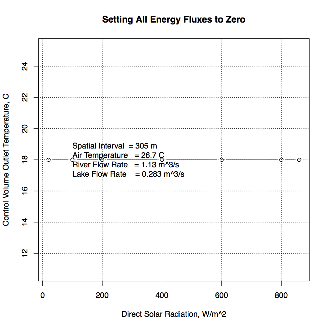
Figure 4. Westhoff et al. Model - All External Energy Sources and Sinks Set to Zero.
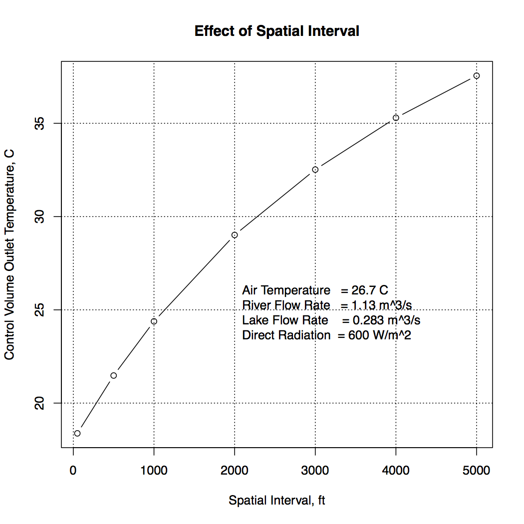
Figure 5. Westhoff et al. Model - Changing the Spatial Interval Size.
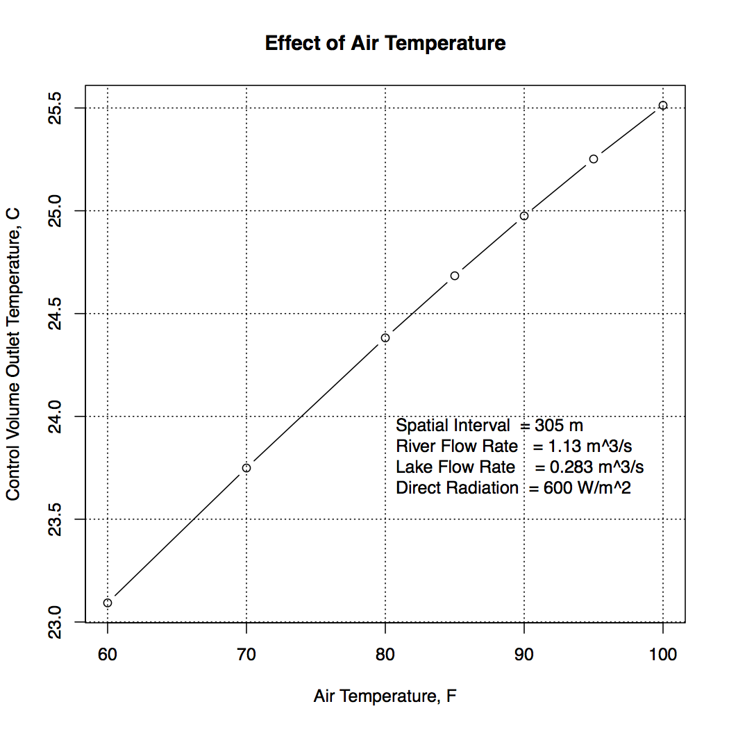
Figure 6. Westhoff et al. Model - Changing the Air Temperature.
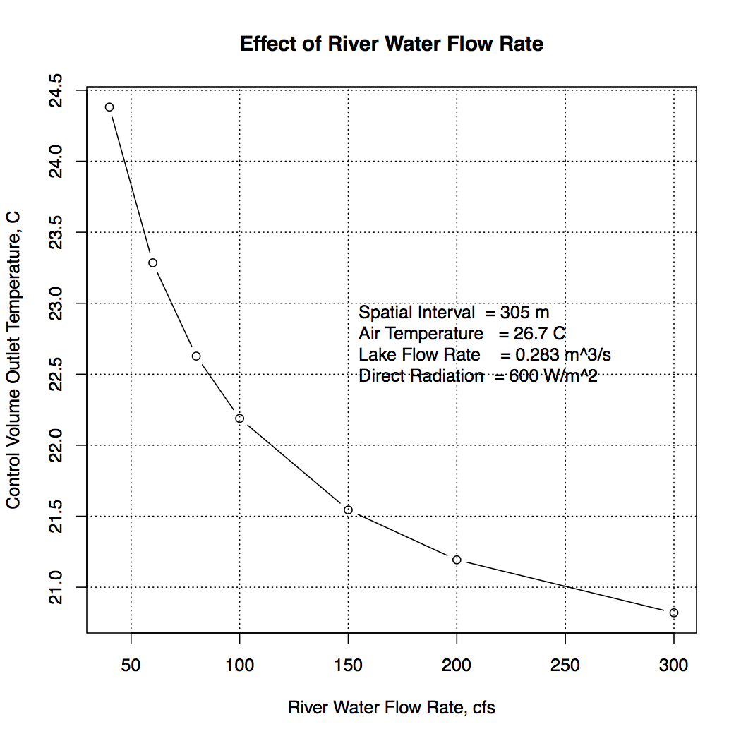
Figure 7. Westhoff et al. Model - Changing the River Water Flow Rate.
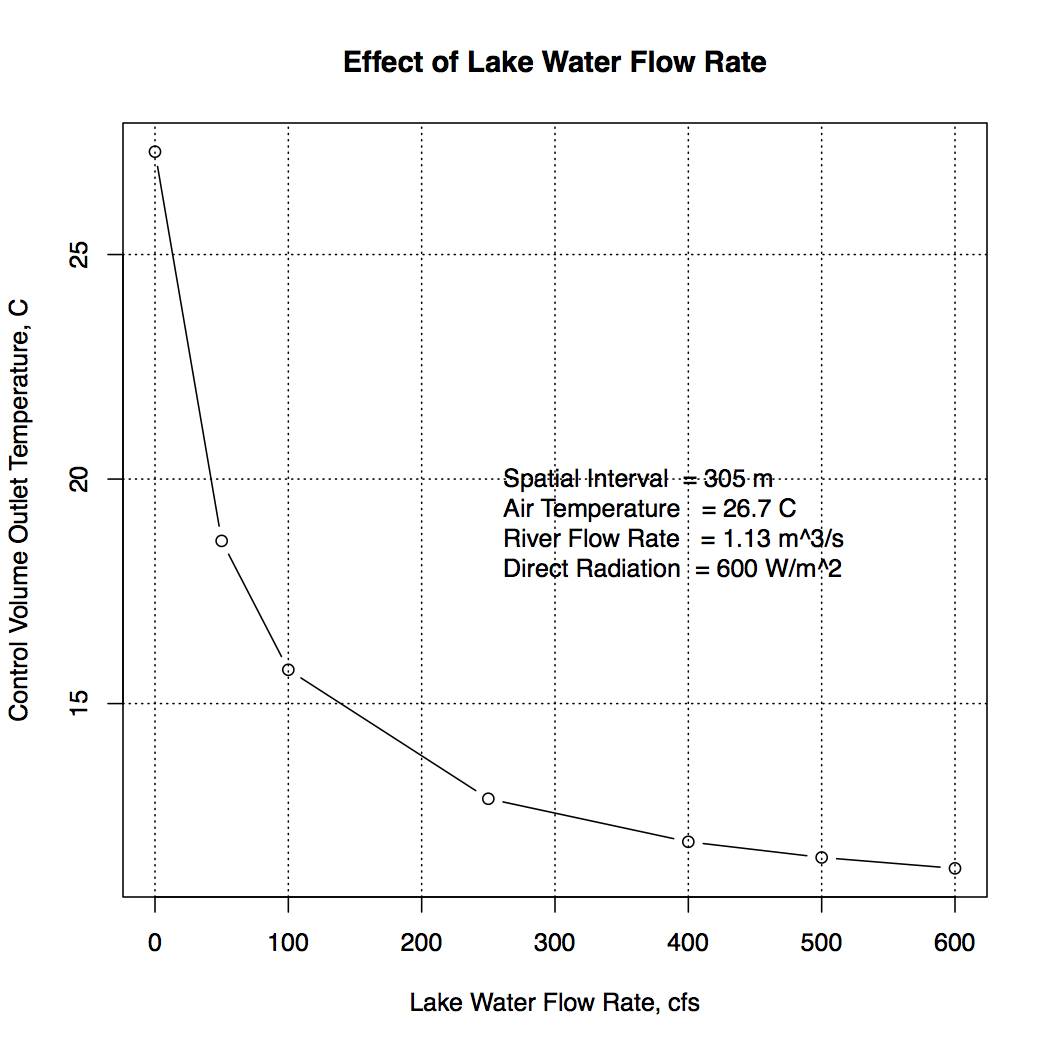
Figure 8. Westhoff et al. Model - Changing the Lake Water Flow Rate.
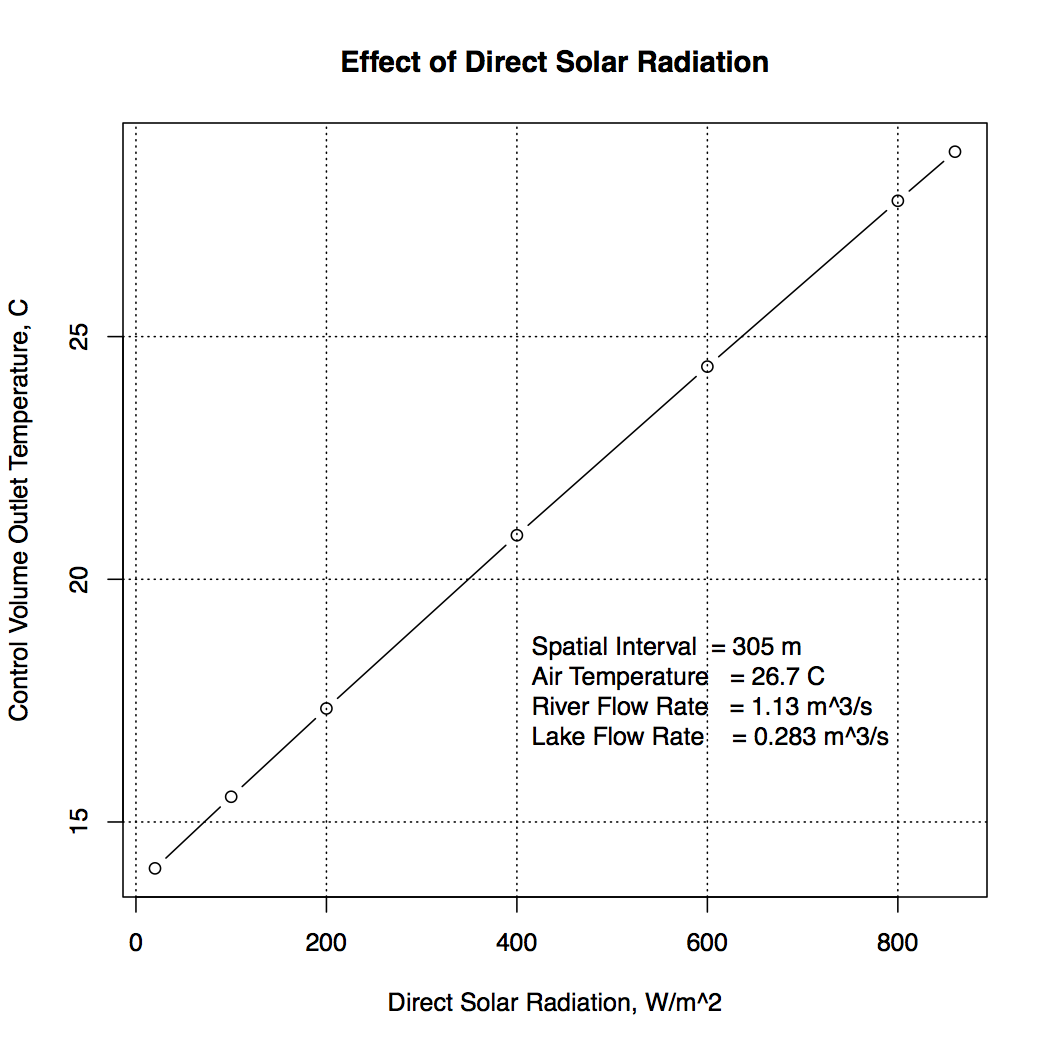
Figure 9. Westhoff et al. Model - Changing the Solar Radiation of a 1,000 ft Interval.
References 4 - 9 provide additional insightful background material to the current problem. There are many others.
In this part of the discussion on TER I will attempt to developed the rudiments of a full-fledged model. I don’t have the resources to get accurate geometric data of the Youghiogheny River, and therefore will make some, hopefully reasonable, assumptions that are based on values found in the literature.
Much of the desired information exists thanks to a careful study conducted by Penelec and reported in extensive documentation in 1994., which will be referred to from now on is the Penelec Study.
The following items are obtained from that Penelec Study and will be placed in a form suitable for a computer model.
The first item is the stretch of river under consideration. This is from Figure 1 above [Penelec Study, p.]. The stretch of the river under considerations is between the red circles, from the Hydroelectric facility’s tail race to the Sang Run river bridge. This figure can be used to estimated the segmentation (making of control volumes) and the shading factors for the river banks because of the orientation of the river segment with respect to the solar angle.
Figure 10 [Penelec, p 3-145] shows the longitudinal profile of the river. The region of interest is between the red circles. As can be seen, the river drops very gradually, so that acceleration effects are going to be minimal." >}}
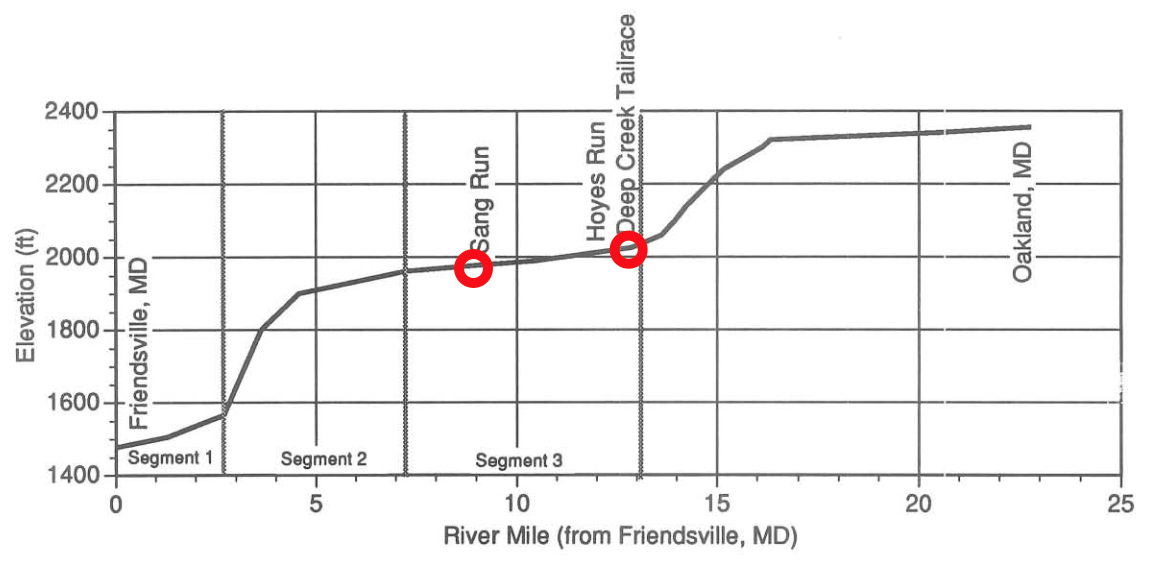
Figure 10. Longitudinal Profile of the Youghiogheny.