Analysis of the Deep Creek Lake (MD) Environment - The Various Problems

1. Scripts Developed to Produce the Bathymetry of the Coves and the Lake

First published PLV: August 20, 2017; Last Updated: August 23, 2017

NOTE: In general, clicking on a graph opens a page with a larger version of it.

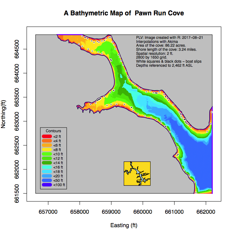
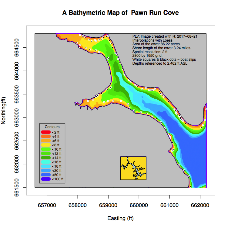
The original bathymetric work was performed in 2012. The result of that work is presented on the deepcreekanswers.com website. The purpose of the work was to identify what boat slips would get into trouble at lower water levels. Getting into trouble means that boats would get stranded when the water level dropped too much because of operations conducted by the Deep Creek Hydro power generating facility. The process on how I got to those maps will be updated and described in detail here.

Originally trying to produce a single bathymetric map of the lake was impossible because the desired resolution, around 5ft or less for a cell size, required a lot of computer memory and the corresponding file size became huge. This also made a single computer run excessive time consuming. Because only certain coves were of interest, it was decided to focus on those coves. The data requirements were less and computer run times were short and hence a lot of trial and error could be conducted to generate the ultimate desired maps. Ultimately, detailed bathymetries were generated for approximately 40 coves or areas of interest.

A number of problems had to be sorted out in the process. The first thing was to define the outline of the lake. That became an issue, because the water depths measured by DNR could only go 3 ft and deeper than the lake level at which the data acquisition vessel was operating (see Figure 1). This raised the problem of how to get the bathymetry for water depths less than 3ft, which of course is what most people were interested in. Because the data collected by DNR were done in an irregular manner (the boat collected its gps location and the corresponding depth as it moved around the lake).

The steps involved in developing the final product, a contour map of a cove, can be summarized as follows:

Back to the Top

2. Getting the Bathymetric Data in Shape

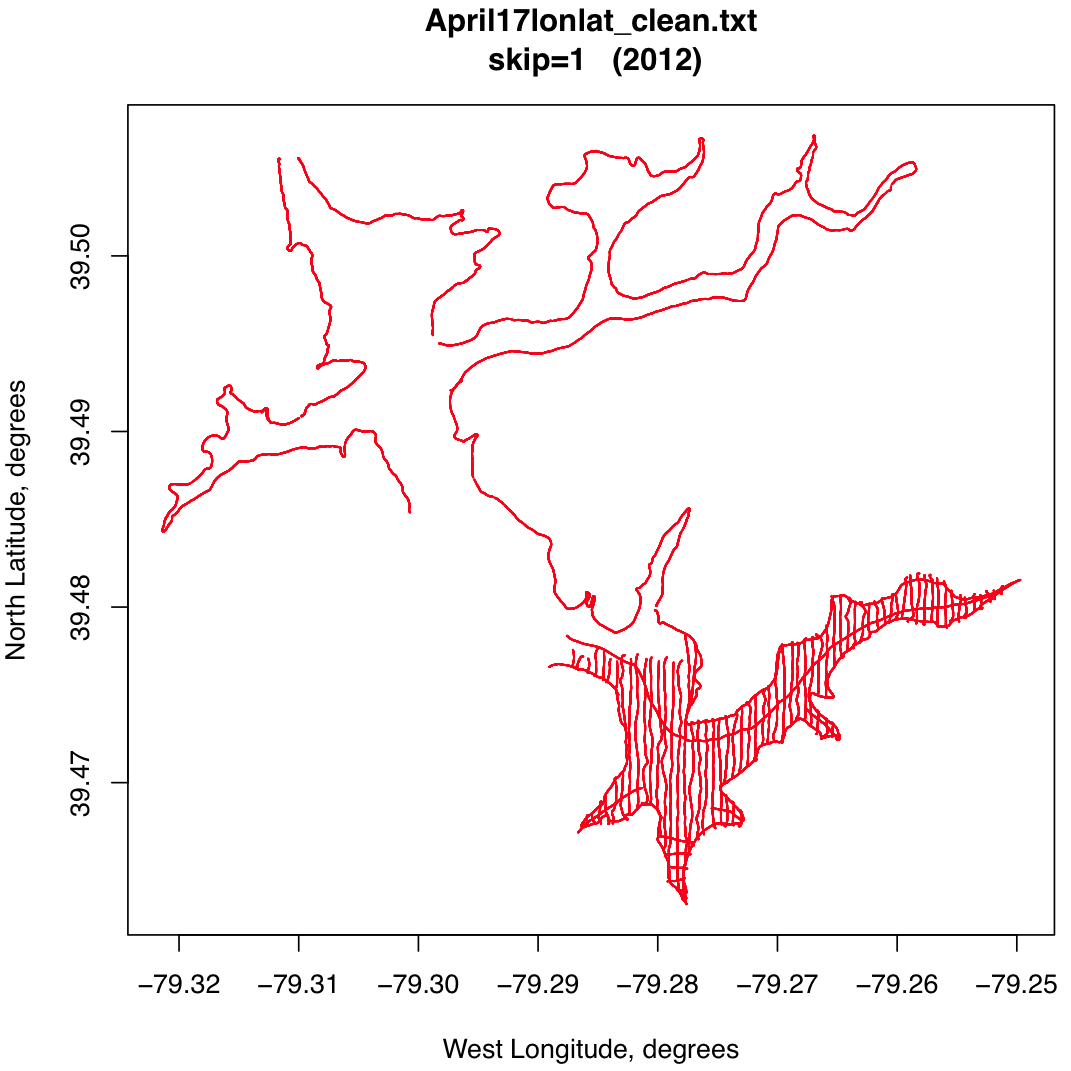
The first step after acquiring the data from DNR in the form of Excel spreadsheets is to convert them to text files that can be processes in various ways and to plot the data to see what we have. This involved writing a very simple script. As mentioned elsewhere DNR took the measurements on April 12, 13, 16, 17, 19, 20, and 21 of 2012. Every measurement taken on April 17 is plotted in Figure 2-1.

Figure 2-1. All Measurements Obtained by DNR on April 17, 2012.

What appear as lines are in reality closely spaced measurements. This is easily verified by plotting every 50th points, with the results shown in Figure 2-2.

Figure 2-2. Plotting Every 50th Measurement Obtained by DNR on April 17, 2012.

The figures for every 10th point are here and for every 100th point here.

Similarly, all of the data for all of the 7 days of measurements are in one file here [3.3 MB]. The files with plots for every 50th point are here. These are pdf's so that they can be enlarged. Note also that these are in latitude/longitude coordinates.

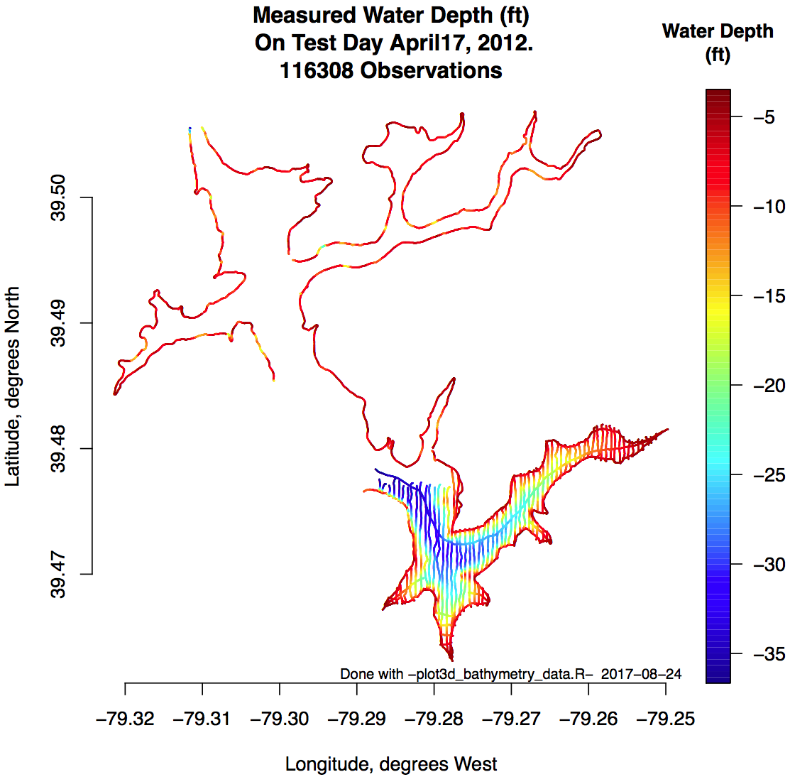
The next thing to do is to find out what kind of depths are associated with this data. Again an R script was written to look at this. Figure 2-3 is an example for the same data as in Figure 2-2. All of the maps can be found here.

Figure 2-3. April 17, 2012 Colored Transects.

Back to the Top

3. Getting an Outline of the Lake

Various plotting and data processing attempts were conducted, but it soon became clear that one needed an outline of the lake as a reference to see how well the data locations were, some kind of well-known boundary condition. Turning to the County I obtained a shape file of the outline of the lake. The pedigree of that outline was unclear, except to say that it was digitized from aerial photographs taken in 2005, roughly the middle of April (exact source and date unknown). It was assumed that the lake level was 2461 ft ASML, and hence the 2012 bathymetric work was based on that assumption. A boundary of the shoreline thusly created is shown in Figure 3-1.

Figure 3-1. The Outline of Deep Creek Lake using the County's Data.

Based on data recently collected, the level in April, 2005 could be as low as 2459.8 or as high as 2460.5. The 2461 was always a nagging question, but based on this later information the real data introduces considerable more uncertainty in the maps at the shallow depths, as shown on deepcreekanswers.com, than previously thought.

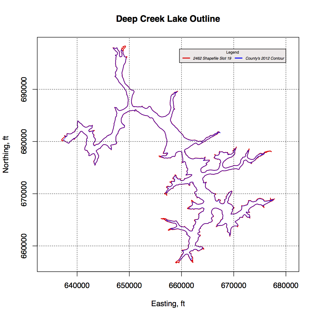
Good data exists in the form of the buy-down maps (see here on the deepcreekanswers.com website) but would be expensive to acquire and/or digitize. Of particular interest was the 2462 surveyed contour line because that elevation coincides with the elevation of the spillway near the dam. Because it is surveyed, the contour line is as near the "truth" as one could possibly get.

I figured that the data must exist in some digital form somewhere, but I could not locate it. Neither the MDE or DNR, who should have it, nor Lake Management, nor the County had the data. After years of on and off searching I finally was able to locate a copy of an AutoCad file containing the 2462 surveyed contour. It took some doing to get the actual coordinates off the proprietary format, but this was eventually accomplished via a web service that was able to convert the file to an ESRI shape file. With "R" I could then process the shape file and extract the coordinates of the 2462 ft contour in meters, and easily transformed to feet. That data file can be downloaded from the deepcreekscience.com website.

A comparison between the assumed 2461 and the 'true' 2462 lake outline can be found in Figure 3-2.

Figure 3-2. Comparing the 2462 Contour Against the Assumed "2461" outline.

Back to the Top

4. The State Plane Coordinate System

The process of establishing a shoreline brought about a new issue for the bathymetric data namely that we had to do define our numbers in terms of the the State Plane Coordinate System. This is a coordinate system for referring to the locations of things used by the State of Maryland and all surveyors by simply specifying an x and y-value. See this Wikipedia article for an overview of the SPCS.

Over the years "R" has become a very powerful spatial data manipulation system; spatial data means defining attributes, such as buildings, roads, signs, etc., at locations on earth. Hence a simple script could be constructed that would transform the latitude/longitude coordinates of the bathymetric data to Northings/Eastings, the term used to designate simple x/y coordinates with respect to some fixed reference an plot them over the the lake shoreline.

A map of the raw data expressed in State Plane Coordinates, enclosed within the new 2462 lake shore line, can be seen in Figure 4-1. The map shows all the points. But, because of the density of the points, they appear as lines in the graph.

Figure 4-1. Raw Data in SPCS.

Back to the Top

5. Cove Boundary DefinitionBathymetry2017->Coves

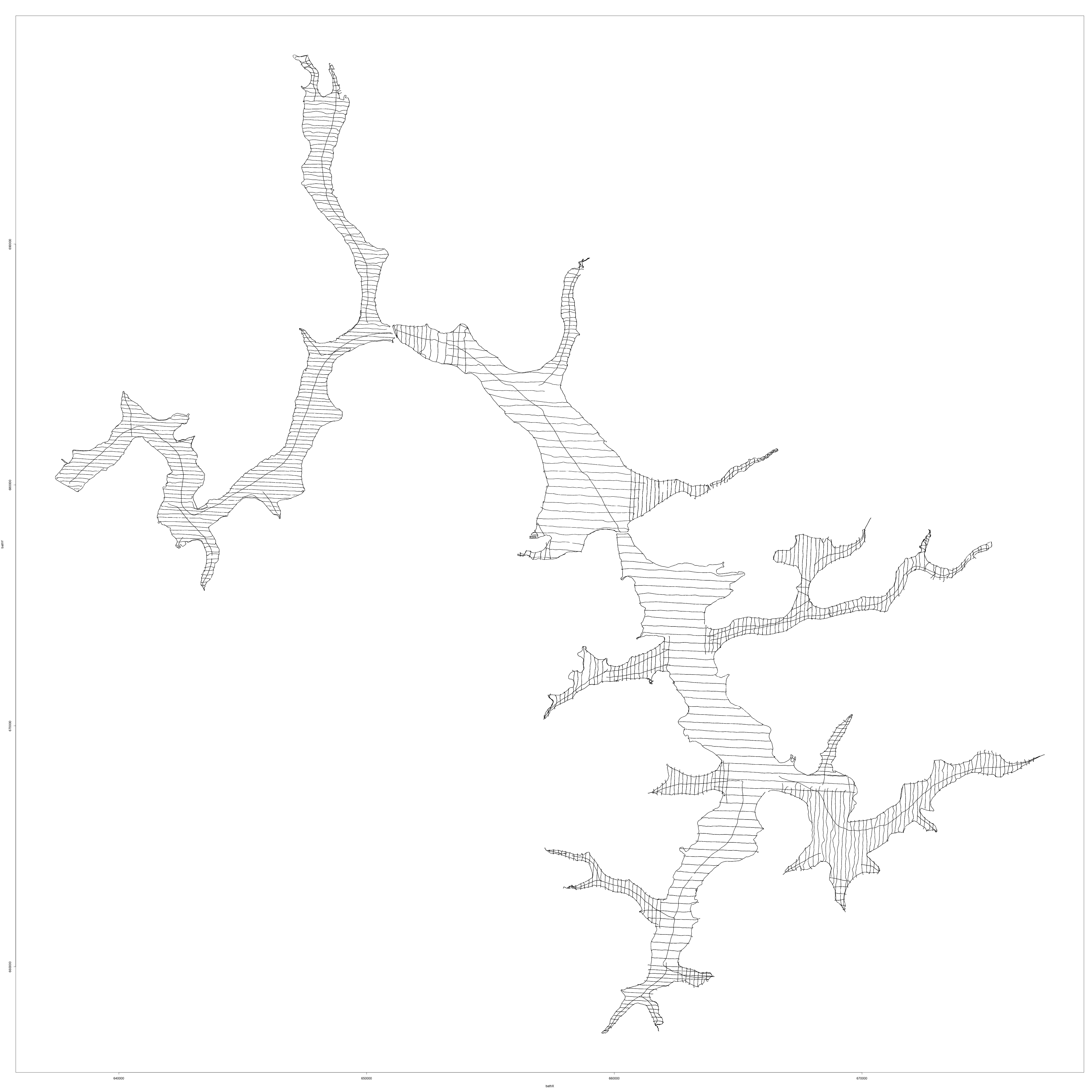
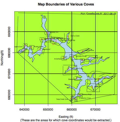
A cove was defined rather arbitrarily by defining a polygon around the cove using Northing/Easting coordinates from a map of the lake. This were defined with a digitizer application. The type of result found is shown in Figure 5-1.

Figure 5-1. Arrowhead Cove Definition Data.

A graph of some of the cove definitions is shown in Figure 5-2.

Figure 5-2. A Presentation of some of the Cove Bounds.

Back to the Top

6. Define the Data Region for the Cove.

Back to the Top

7. Extract the Cove Data from the Master Files

Back to the Top

8. Workflow for Producing the Cove Maps

Once the basic data sets are in place, the workflow is one of production and is a s follows:

Back to the Top

9. Sensitivity Studies

As has been discussed earlier, there are many very closely spaced data points on comparatively widely spaced transects. Hence a parameter has been introduced in the mapping process, mostly to speed up the calculations, that selects only every nth data point. The images below shows the effect on the maps. As one can see, the maps where only every

Back to the Top

10. Interpolating the Data

Gridding irregularly spaced data is a common requirement in the spatial world (Latitude/longitude worlds).

Figure 10-1. Pawn Run Cove Map with Akima Interpolation.

Figure 10-2. Pawn Run Cove Map with Akima-2 Interpolation.

Figure 10-3. Pawn Run Cove Map with Loess Interpolation.

Back to the Top

11. Number of Data Points Used (precision)

Back to the Top

12. Methodology Validation - This work was done in fall of 2012.

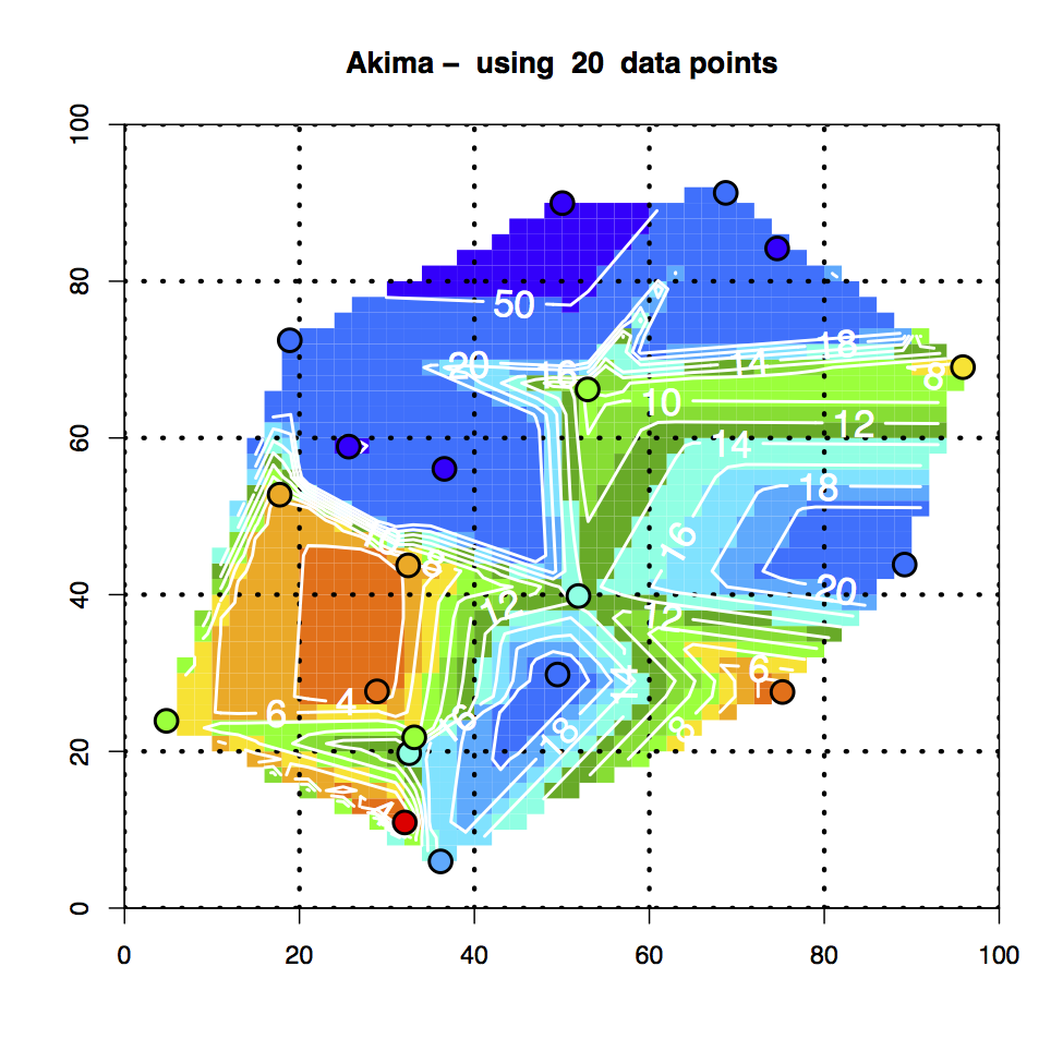
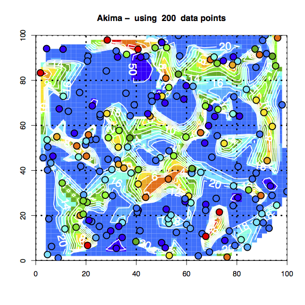
The Akima algorithm is used in the scientific community extensively in all kinds of applications. The question here is:Does it do a good job representing the bathymetry?"

To answer that question I choose to define a test problem, and tried out various ways to demonstrate the “goodness of fit.”

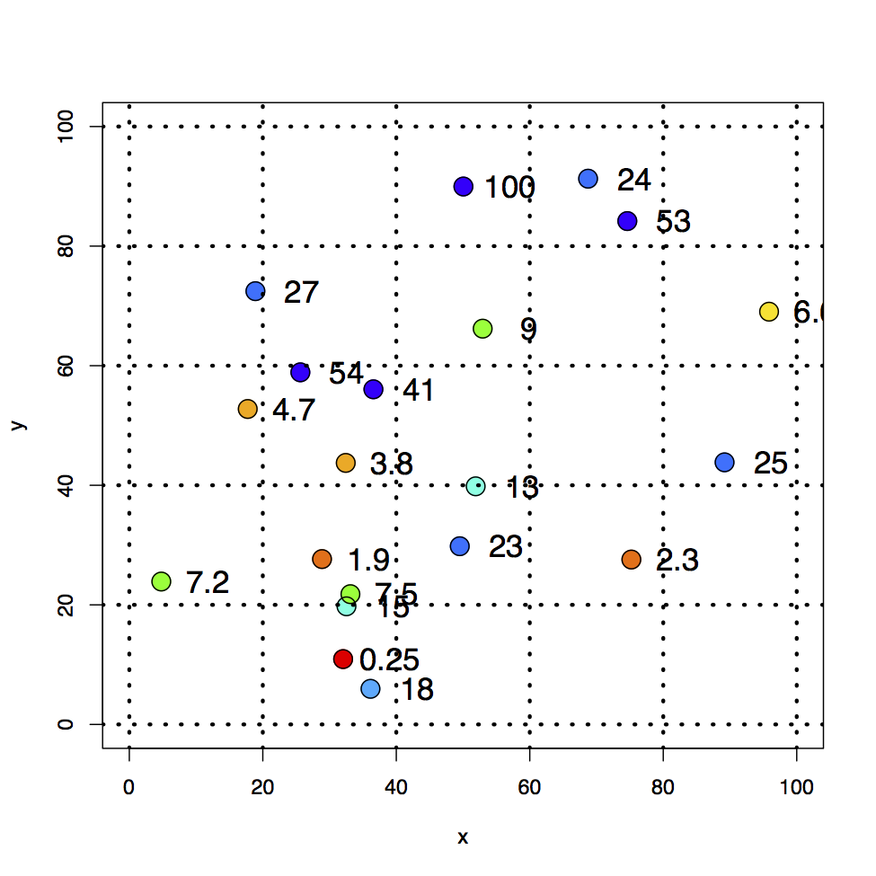
I defined a grid of 100 x100 ft or miles, or whatever; units do not matter. For that grid, I computed a random set of x,y coordinates and z values. For ‘x’ and ‘y’ they were selected from a uniform distribution between 0 and 100, for ‘z’ they were selected from a normal distribution with the resulting values normalized to 100, equivalent to the maximum depth value used in all of the bathymetric work.

I used the same color palette and breaks in water depth levels that were used to generate the final bathymetry map.

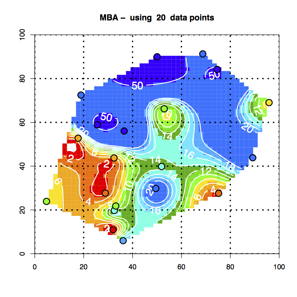
In addition to the Akima interpolation procedure, I recently found another method in one of the R packages, labeled as MBA (R has thousands of functions collected in hundreds of packages and, because of the sheer number of them, its easy to miss some very useful ones).

The result of this analysis is basically four graphs:

1. A bar graph showing the colors and range of the color coding as provided by the palette used.
2. A scatter plot with just the color coded ‘z’ points. Note that the values of the points are also shown.
3. A graph with the Akima interpolation results and the color coded points super imposed.
4. A graph with the MBA interpolation results similar to the Akima one.

An additional pair of images was run with a 10 fold increase of data points and the results shown in Figure 12-5.

Figure 12-1. The color palette used. The numbers below the bars signify the end of the bar interval. Hence ‘2’ means it goes from 0 to 2; 50 means it goes from 20 to 50..

Figure 12-2. The points are color coded according to the color palette shown in Figure 1. The numbers next to the points are the z-values.

Figure 12-3. This graph shows the results of the Akima interpolation method. Whether the shapes of the contours are right or wrong can be debated. They do lie, more or less, where one expects them to be. In other words, the points appear to lie in their appropriate locations.

Figure 12-4. This graph show the results of the MBA interpolation method. The contours are much more pleasing to look at. The points also fall on the correct locations. These results compare reasonably well with the Akima results, but they are different.

Back to the Top

Figure 12-5. This this figure the number of data points have been increased 10 fold, from 20 to 200.

Back to the Top

13. Final Maps

Back to the Top