Piet's Notes on Deep Creek Lake Science
Sensible Technologies - The Science of Deep Creek Lake
This note is a description of how one can make an aesthetically pleasing graph by masking out unwanted elements.
This is about making nicer bathymetry plots with “R”. Coves have an irregular geometry. As a result, for example, when fitting bathymetric data to a function, the math introduces spurious results outside the boundaries of the cove. These results have no meaning with respect to contours. The lake shoreline is a “zero” water depth contour, is supplied when doing the bathymetry, and the contour functions should pass through that. Hence anything outside the lake shoreline contour can be covered up by white or any other desired color. On top of tst one could plot roads and structures and mountain ranges, whatever one desires.
[The spurious/extraneous information is seen when one plots the results.]({{ < ref “/methods/html/TestProblem.html” > }}) To generate an aesthetically pleasing plot these extraneous results should be covered up by some kind of single color or other mappings. This is called “applying a mask.”
As it turns out, “R” does not have a suitable masking function, or at least I can’t find a properly working one. This note is about creating my own version of a masking function that works for my purposes.
To demonstrate the concept and solution, I’ve put together a sample problem that mimics the conditions. The problem used for the development process is a diamond with a rectangular hole and a set of points of which some are masked off.
“R” defines a plot area on which a graph is generated. The plot area is on a background. All kinds of items can be controlled by settings and functions.
The plot area is defined by a bounding box placed on a background. The sample points are plotted there, as seen in Figure 1. Superimposed we have a couple of polygons, one that defines backdrop, and one that defines a window through we should be able to see all data points except the ones falling on this second backdrop.
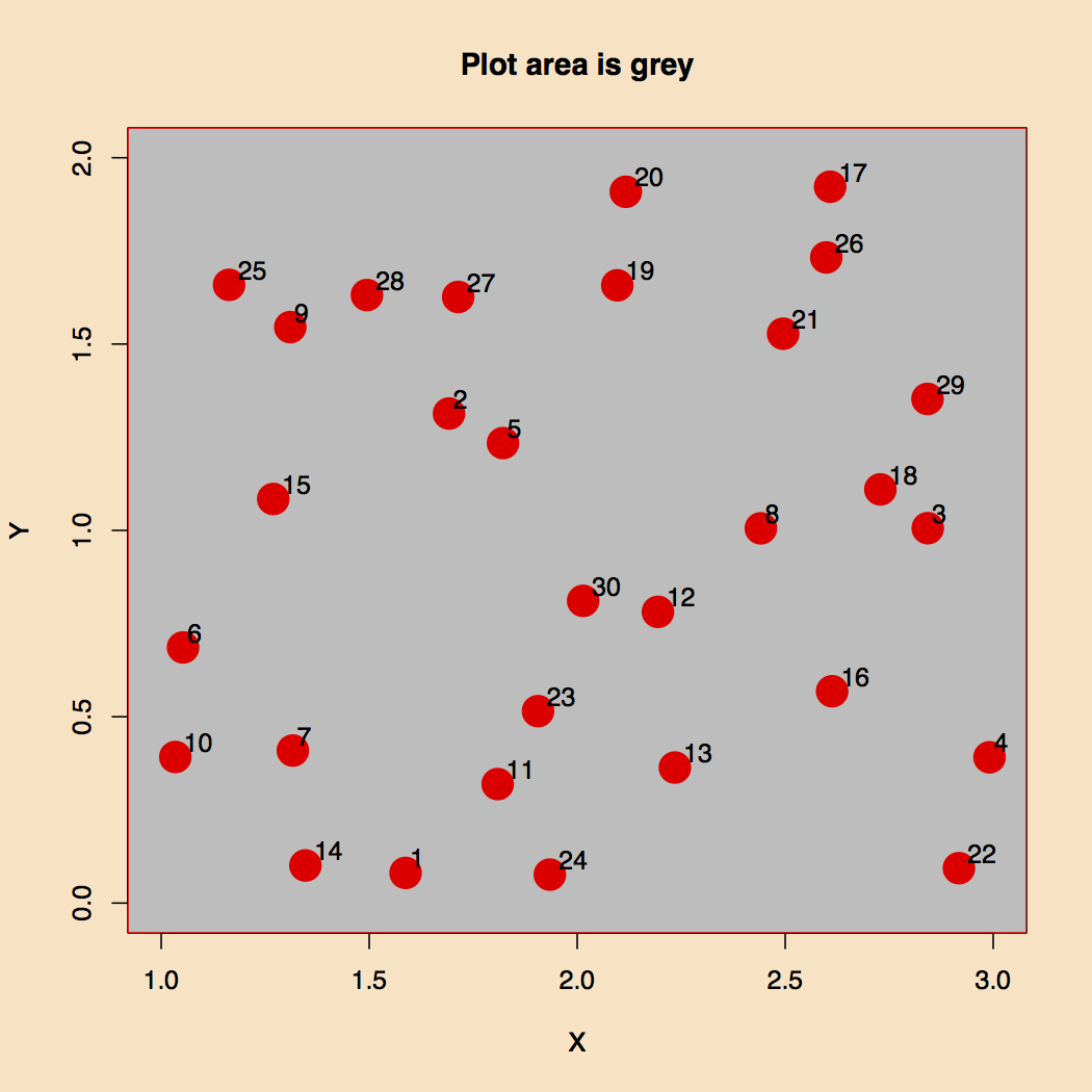
Figure 1. Background and Plot Area.
Here are definitions of the bounding box, p1, two areas, p1 and p2, and the number of random coordinate sets, nc. I had to go up to 30 random points in order for some to show up in the window.
p0 <- rbind(c(1, 0),  c(3, 2))    # The bounding box or extent
p1 <- rbind(c(1.0, 1.0),  c(2.0, 0.0),  c(3.0, 1.0),   c(2.0, 2.0), c(1.0, 1.0))    # The square
p2 <- rbind(c(1.5, 0.75), c(2.5, 0.75), c(2.5, 1.25), c(1.5, 1.25), c(1.5, 0.75))   # The rectangle
nc <- 30   # The number of test sample coordinates
Figure 2 plots the points and the two closed polygons. The idea is to make a polygon such that only points 5, 8, 12 and 30 show in the inner rectangle and other points outside the outer polygon.
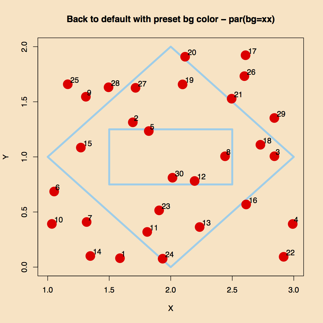
Figure 2. Polygons and Points.
To make this work one must understand how polygon drawing algorithms work. In this case the inner rectangle is defined by points that start on the lower left hand corner and go clockwise. The same was done with the outer polygon. The strategy is to draw one polygon. So in order to get out of the inner polygon one has to start traveling in the opposite direction which would now be clockwise. To make the polygon drawing algorithm work one must start the inner one going clockwise.
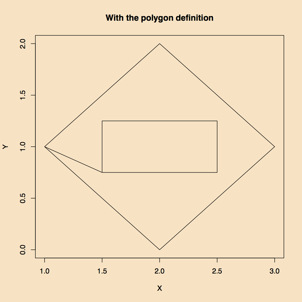
Figure 3. How to Make Two Polygons into One.
This methodology has been incorporated into a couple of functions.
# The following function determines whether a dataframe of x any is clockwise or counter-clockwise
# If the result is positive, it is clock-wise.  If it's negative it's counter clock-wise
# REF: https://stackoverflow.com/questions/1165647/how-to-determine-if-a-list-of-polygon-points-are-in-clockwise-order
# Assumes Cartesian coordinates
# Formula only works for CLOSED polygons.
point_order <- function(df){
	x <- df[[1]]
	y <- df[[2]]
	n <- length(x)
	sum <- 0
	for(i in 2:n){
		sum <- sum + (x[i]-x[i-1])*(y[i]+y[i-1])
	}
	sum
}

# The following function makes one closed polygon in such a way that the one defined by df1
# becomes a transparent window inside df2,
# where df1 and df2 are dataframes defining closed polygons.
hole_in_frame <- function(df1, df2){
	q1 <- df1
	q2 <- df2
	s1 <- point_order(df1)
	s2 <- point_order(df2)
	# If TRUE we have to reverse one of the data sets
	if(s1 > 0 && s2 > 0 || s1 < 0 && s2 < 0) {
		q1 <- q1[order(nrow(q1):1), ]    #invert row order
	}
	# We now put the two dataframes together
	q3 <- rbind(q1, q2)
}
The result, shown in Figure 4, is as one hoped for.
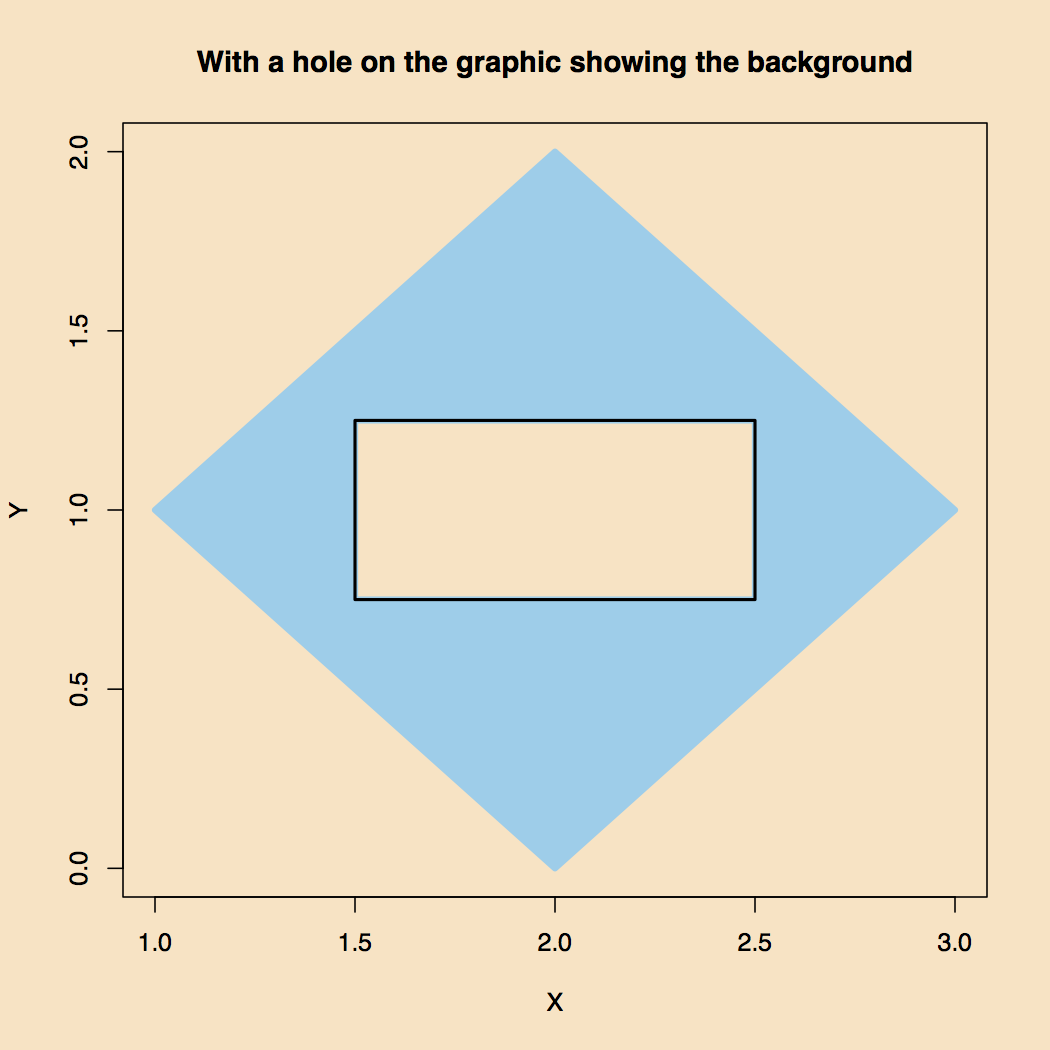
Figure 4. A Transparent Window into the Second Polygon.
To put all this together requires the following “R” code:
# Everything, including the points showing through and around
plot(p1, type="n", xlab="", ylab="")
points(cords, pch=20, col="red", cex=4)
textxy(cords$x, cords$y, ptlabs, cex=1)  # Requires package 'textxy'
q3 <- hole_in_frame(q1, q2)
polygon(q3$X1, q3$X2, col="skyblue")     # Requires package 'Polygon'
lines(q3$X1, q3$X2, col="skyblue", lwd=4)
points(q2, type="l", lwd=2)
title(main="The Whole Works", xlab="X", ylab="Y")
These eight lines of code do the following:
The final result of this effort is shown in Figure 5.
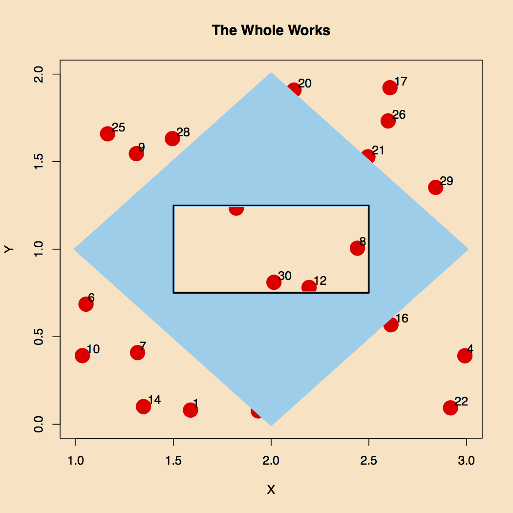
Figure 5. The Final Result.
The working pieces of this work are put in a set of two functions that are easily called by a main script. These functions are shown in the next section of code.
point_order <- function(dff){
	x <- dff[[1]]
	y <- dff[[2]]
	n <- length(x)
	sum <- 0
	for(i in 2:n){
		sum <- sum + (x[i]-x[i-1])*(y[i]+y[i-1])
	}
	sum
}

hole_in_frame <- function(df1, df2){
	# Force the names of the two data frames to be the same
	q1 <- df1
	names(q1) <- c("X", "Y")
	q2 <- df2
	names(q2) <- c("X", "Y")
	s1 <- point_order(q1)
	s2 <- point_order(q2)
	# If TRUE we have to reverse one of the data sets
	if(s1 > 0 && s2 > 0 || s1 < 0 && s2 < 0) {
		q1 <- q1[order(nrow(q1):1), ]    #invert row order
	}
	q2 <- rbind(q2, q1[nrow(q1),])
	# We now put the two data frames together
	q3 <- rbind(q1, q2)
	return(q3)
}
These functions come with the following usage description:
Usage:
1) Define two polygons with x/y coordinates, q1 and q2, where q1 is the hole
2) Place in the main script: source(../functions/hole_in_frame.R)
3) Call: q3 <- q3 <- hole_in_frame(q1, q2)
4) Make sure to have loaded 'library(sp)'
5) After plotting interpolated output: polygon(q3[[1]], q3[[2]], col="grey") # Any color
Have fun….