Piet's Notes on Deep Creek Lake Science
Sensible Technologies - The Science of Deep Creek Lake
The Akima method of interpolation 2-D and 3-D scattered data has been used for all of the bathymetry work described on this website. Here I try to describe what it is and how I used it.
From the R documention this is what it says:
Gridded Bivariate Interpolation for Irregular Data
Description
These functions implement bivariate interpolation onto a grid for irregularly spaced input data. Bilinear or bicubic spline interpolation is applied using different versions of algorithms from Akima.
Usage
interp(x, y=NULL, z, xo=seq(min(x), max(x), length = nx),
yo=seq(min(y), max(y), length = ny),
linear = TRUE, extrap=FALSE, duplicate = “error”, dupfun = NULL,
nx = 40, ny = 40,
jitter = 10^-12, jitter.iter = 6, jitter.random = FALSE)
The first three variables are basically the x, y, and z values of the scattered points. Alternative one can provide a SpatialPointsDataFrame object.
xo = vector of x-coordinates of output grid. The default is 40 points evenly spaced over the range of x
nx = number of equally spaced grid-points in the x-direction
yo = vector of y-coordinates of output grid. The default is 40 points evenly spaced over the range of y
ny = number of equally spaced grid-points in the y-direction
linear is a logical variable indicating bilinear interpolation. If TRUE it’s a bicubic spline interpolation.
The output is an x/y grid with interpolated z values from which contours are generated.
There are some other setting that basically take care of duplicate data. I have not found them to be needed.
Figure 1, 2 and 3 show the results from one of the data sets that is available via the ‘akima’ package. The data package includes five test sets that were originally put together by Franke as a testbed for his development efforts. The data sets are also described here.
Figure 1 uses the default gridspacing of 40 intervals with bilinear interpolation.
Figure 2 is with 200 grid points in both x and y direction and bilinear interpolation.
Figure 3 is as Figure 2 but with bicubic spline interpolation. As can be seen the spline method gives more pleasing results.
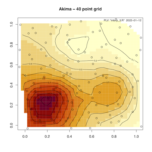
Figure 1 - With default grid spacing (40 point).
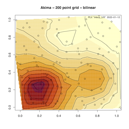
Figure 2 - With 200 point grid spacing - bilinear interpolation
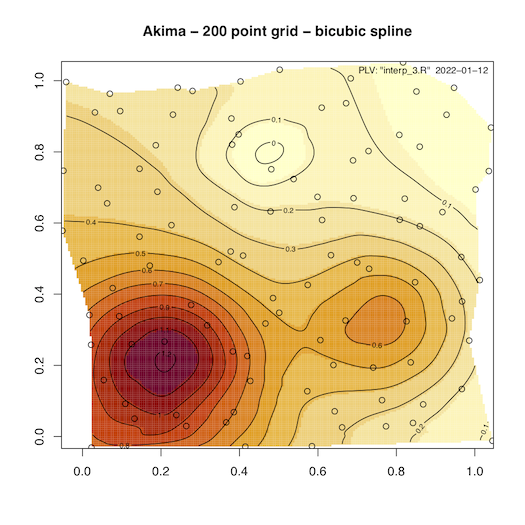
Figure 3 - With 200 point grid spacing - bicubic spline interpolation
The full script that generated the images in this note can be found here.