Piet's Notes on Deep Creek Lake Science
Sensible Technologies - The Science of Deep Creek Lake
The process of establishing a shoreline brought about a new issue for developing a bathymetric map of the lake, namely what coordinate system to use. Pretty much all issues dealing with surveying, and hence by extension, bathymetric analyses are put in terms of the the State Plane Coordinate System (SPCS).
This is a coordinate system for referring to the locations of things used by all states, including the State of Maryland, and most surveyors, by simply specifying an x- and y-value. See this Wikipedia article for an overview of the SPCS.
Over the years “R” has become a very powerful spatial data manipulation system; spatial data means defining attributes, such as buildings, roads, signs, etc., at locations on earth. A simple script can transform the latitude/longitude coordinates of the bathymetric data to Northings/Eastings, the term used to designate simple x/y coordinates with respect to some fixed reference, and plot them together with the lake shoreline.
A map of the raw data expressed in State Plane Coordinates, enclosed within the new 2462 lake shore line, can be seen in Figure 1. The map shows all the points that are available (the lines are actually closed spaced points). But, because of the density of the points, they appear as lines in the graph.
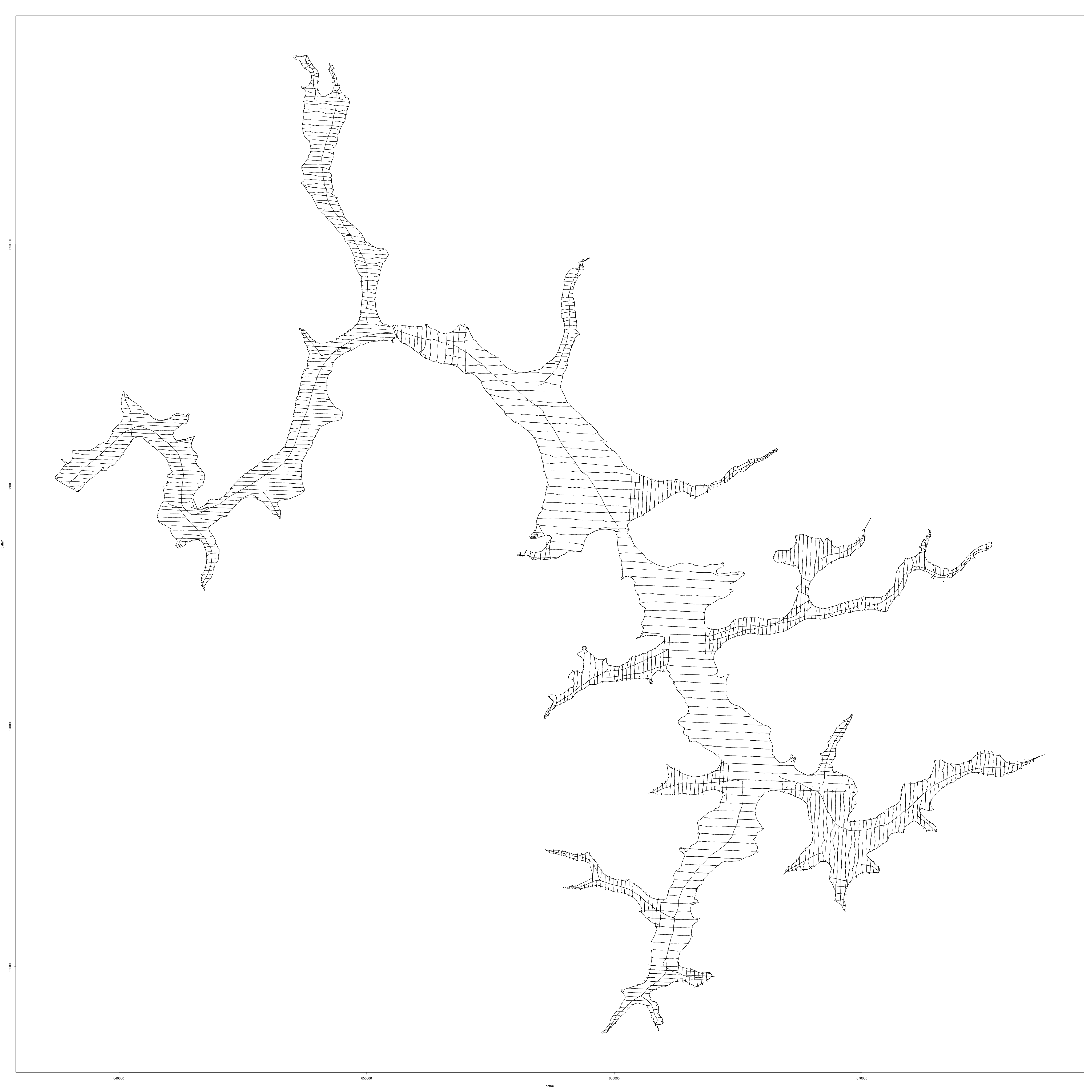
Figure 1. An Example of Mapping ALL Raw Data.
To be able to do this required an understanding of SPCS which was accomplished with a lot of googling. The result of this is a collection of unstructured information that allowed me to convert and make usable, in R, coordinates from Latitude/Longitude to UTM and the Maryland State Plane Coordinate System.
The State Plane Coordinate System (SPCS) is not a projection; rather it is a system for specifying positions of geodetic stations using plane rectangular coordinates. This coordinate system that divides all fifty states of the United States, Puerto Rico and the U.S. Virgin Islands into over 120 numbered sections, referred to as zones. Each zone has an assigned code number that defines the projection parameters for the region.
The main aim in creating the SPCS was to design a conformal mapping system for the entire country while maintaining a maximum scale distortion of 1 part in 10,000. In 1933 this was considered the limit of surveying accuracy. In order to attain this accuracy, the larger states needed to be divided into smaller zones or FIPS. Each zone or FIPS has its own central meridian or standard parallels to maintain accuracy.
The original zones were based upon a network of geodetic control points known as the North American Datum of 1927 (NAD27). With improvements within the last 50 years and the need for compatibility with satellite systems, the origin of the datum was moved and NAD83 was created. Hence ZONE refers to the older NAD27 system and FIPSZone to the newer NAD83.
Most state plane zones are based on either a transverse Mercator projection or a Lambert conformal conic projection.
FIPS = Federal Information Processing Standard
Typical coordinate values I got from the County and DNR
638486.2      679792.4
!!!!Concluded that these numbers are in MD State plane coordinates and in ft!!!!
From Rich From Ort and Google Earth/Excel Conversion; these come out as UTM coordinates
4371866.21	644380.86

MD023(GARRETT CO.) NAD83 ZONE = 1900 (LAMBERT|ONLY A SINGLE ZONE FOR THIS STATE OR COUNTRY)

MARYLAND FIPSZONE: 1900 ADSZONE: 4126 UTM ZONES: 17 & 18

esri:102285 is the Maryland State Plane for NAD 83 with units in meters

epsg:4326 is the standard longitude/latitude coordinate system

WGS84 Bounds: -79.8443, 36.2557, -73.3843, 42.2065

```
PROJCS["NAD_1983_StatePlane_Maryland_FIPS_1900_Feet",
    GEOGCS["GCS_North_American_1983",
        DATUM["D_North_American_1983",
            SPHEROID["GRS_1980",6378137.0,298.257222101]],
        PRIMEM["Greenwich",0.0],
        UNIT["Degree",0.0174532925199433]],
    PROJECTION["Lambert_Conformal_Conic"],
    PARAMETER["False_Easting",1312333.333333333],
    PARAMETER["False_Northing",0.0],
    PARAMETER["Central_Meridian",-77.0],
    PARAMETER["Standard_Parallel_1",38.3],
    PARAMETER["Standard_Parallel_2",39.45],
    PARAMETER["Latitude_Of_Origin",37.66666666666666],
    UNIT["Foot_US",0.3048006096012192]]
Deep Creek Lake
 79°18'56.63"W	-79.31573056
 39°30'31.66"N	39.50879444

 =======================================================
           Latitude           Longitude      Datum Zone
 INPUT =   N393031.66         W0791856.63    NAD83 1900
 =======================================================

  NORTH(Y)    EAST(X)     AREA  CONVERGENCE   SCALE
  METERS      METERS            DD MM SS.ss
  ----------- ----------- ----  -----------   ----------
  207017.263  200860.407  MD    -1 27 12.35   1.00001081


  Rockville
  Latitude:  39° 05' 02" N
  Longitude:  077° 09' 11" W

  =======================================================
            Latitude           Longitude      Datum Zone
  INPUT =   N390502.0          W0770911.0     NAD83 1900
  =======================================================

   NORTH(Y)    EAST(X)     AREA  CONVERGENCE   SCALE
   METERS      METERS            DD MM SS.ss
   ----------- ----------- ----  -----------   ----------
   157329.915  386757.601  MD    -0  5 45.83   0.99995642
“The United States survey foot is defined exactly as 1200⁄3937 meter, approximately 0.3048006096 m” -> or 1 m = 3.280833333 ft One usually finds: 0.3048 m -> or 1 m = 3.280839895 ft
Beginning July 1959 the length of the international yard in the United States and countries of the Commonwealth of Nations was defined as 0.9144 meter. Consequently, the international foot is defined to be equal to exactly 0.3048 meter.
An example of applying this knowhow to convert Google Earth lat/lon coordinates of the locations of a sample boat slip file is shown in the following script.
# transform_spsc.R
# PLV: 9/19/2017

# Load the library that defines spatial objects
library(sp)

# Read a sample of the digitized boat slip locations via Google Earth as a data frame
data <- read.table ("../data/sample_boat_slips.txt", skip=1, header=FALSE, sep="\t")

# Assign names to the columns in the data frame
names(data) <- c("Longitude", "Latitude", "Zero", "UTM-Easting", "UTM-Northing", "Zone")

# Converts 'data' to a spatial data object
coordinates(data) <- ~ Longitude + Latitude

# The coordinates are in WGS 84 -> 4326
proj4string(data) <- CRS("+init=epsg:4326")
# See: http://www.geotoolkit.org/modules/referencing/supported-codes.html for coordinates codes
# See also: http://www.epsg-registry.org/

# FIPS (SPCS ID) 1900 -> EPSG ID 26985 (m) -> 2893 (ft) MD
# http://www.eye4software.com/resources/stateplane/
# Convert to Maryland State Plane Coordinates
boatslips <- spTransform(data, CRS("+init=epsg:2893"))

# Extract the SPC and convert to dataframe)
df2 <- data.frame(boatslips@coords)

# Plot the sample of boat slip coordinates in SPCS
plot(df2, type="p", pch=19, col="red")
# Apply a grid to the plot
grid(col="black")
PLV
First Published: 9/18/2017
The scripts associated with this post can be found here.