Piet's Notes on Deep Creek Lake Science
Sensible Technologies - The Science of Deep Creek Lake
Knowing how deep the water is at any given water level can be very important for some folks, especially during a dry year and when one lives in one of the shallow coves. This is because boats may become stranded. Sedimentation in shallow coves has, over the years, become a concern.
To that end, to determine the scope of the problem, DNR conducted a bathymetric survey of the lake in 2012. From that data I produced a series of maps for various coves around the lake, showing the water depth in relation to the height of the spillway near the dam. These maps can be found on the deepcreekanswers.com website. An example of such a bathymetric map is the one shown in thew image below. This is a map of the cove at Arrowhead, showing with color how deep the water is in reference to the height of the spillway, which is at 2462 above sea-level. The blues are deeper, and the more red is shallow.
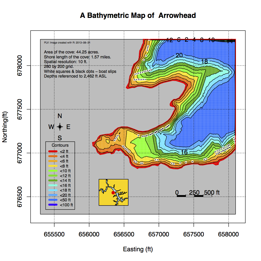
Figure 1. Bathymetry at Arrowhead Cove.
Something was always nagging me when I produced the bathymetric maps in 2012, namely that I did not have a well-documented lake shoreline as a reference and boundary condition when calculating all of the depths. As a result there is some uncertainty in the maps, generally probably very small, 0.5 ft or less perhaps, and mostly in the shallow areas, but not something that could be verified.
Good data exists in the form of the buy-down maps see here on the deepcreekanswers.com website but would be expensive to acquire and/or digitize. Of particular interest was the 2462 surveyed contour line because that elevation coincides with the elevation of the spillway next to the dam. Because it is surveyed, the contour line is as near the “truth” as one could get.
After years of searching I finally obtained a copy of an AutoCad file containing that contour. It took some doing to get the actual coordinates off the proprietary format, but this was eventually accomplished via a web service that converted the file to an ESRI shape file. With “R” I could process the shape file and extract the coordinates of the 2462 ft contour.
This page describes the various I efforts I went through while recreating the bathymetry of the coves and the lake with the 2462 contour line as a boundary condition.On a separate page I provide and explain the scripts that I wrote in the process.
As it turned out, the differences between the more accurate 2462 contour line and the assumed 2461 County line, on a grand scale, are small, but probably significant in shallow areas. The comparison of the “exact” 2462 contour, with the “guessed (County)” 2461 contour is shown in Figure 1. As one can see, they compare very well. When one enlarges the pdf file (you have to download it) one can see that the County shoreline is contained within the 2462 contour, as one would expect.
The data file of the 2462 contour can be found on the deepcreekscience.com website.
The data is in the form of Maryland Easting and Northing ft coordinates. This is a transformation from latitude-longitude points to the Maryland State Plane coordinate system (MD SPCS). This is the standard way to define locations in Maryland. For more detail see the Maryland Geological Survey Coordinates User’s Guideand Ref [2].
1. Nearest neighborhood method (NN) The nearest neighborhood method (NN) assigns the value from the nearest observation to a certain grid cell.
2. Inverse distance weighting (IDW) The method of inverse distance weighting (IDW) is an advanced nearest neighbor approach. The value of a certain grid cell is obtained from a linear combination of the surrounding locations. This method is based on the assumption that the weight of each observation declines with distance.
3. Polynomial functions – splines (SPL) The method of splines (SPL) is based on polynomial functions that fit trends through the observation points by x-order polynomials.
4. Hypsometric method (HYP) The hypsometric method (HYP) is a composite approach which takes account of catchment topography.
5. Kriging (KRI) The probabilistic approach of Kriging (KRI) incorporates the concepts of randomness, linear regression model, geo-statistics and optimum interpolation That method is considered to be the best interpolation technique in case of relatively sparse point data.
1. State Plane Coordinate System; Accessed 8/15/2017.
2. Spatial Reference List; Accessed 8/15/2017.
3. Current Permit (01-Jun-2011) - BROOKFIELD POWER PINEY & DEEP CREEK LLC, GA1992S009(08), MDE
PLV: First Released: 12/12/2012