Piet's Notes on Deep Creek Lake Science
Sensible Technologies - The Science of Deep Creek Lake
For many years now (Dec 2016) I’ve been working with R, a computer language that caught my interest around 2011. Its free, is under active development and has a worldwide following. In other words, a language that one should pay attention to. As it turns out, after using it for many years, R can do a lot of things easily, over a broad line of subject matter.
It was not until bathymetric data of Deep Creek Lake were collected by DNR in the spring of 2012 and when people were expressing interest in how water depth mights vary over the season at their boat slip locations, that I began to seriously explore R to understand how that language could possibly be used to generate bathymetric maps and how to exploit these maps. Before that I was toying with ArcInfo, but the computer resources needed and the cost of the software pushed me over the edge to learn R. And after-all, what’s another language after having worked with Fortran, C++, Python, Ruby, HTML, CSS, PHP, and others. I did conclude that R had all the necessary capabilities to generate beautiful maps and do the heavy numerical cranking. After all, I have always used computers to solve problems. My websites are created manually, mostly with HTML, CSS, and PHP. I’m now also using Markdown.
Back to the bathymetry. I was basically looking for the following capabilities:
1. Have the ability to convert unequally spaced measurements of depth to values on a regularly spaced grid in order to produce contours of depth, e.g., lines of constant depth.
2. Be able to work with geographic, e.g. latitude/longitude, formatted data and convert them to the State Plane Coordinate System.
3. Be able to produce visually pleasing, publication type, maps/graphs/diagrams of the results.
The starting point of my really delving into R consisted of two events:
1. In early 2012, Morgan France and I critically reviewed a work statement prepared by DNR to do the bathymetry of the Deep Creek Lake. DNR did take note of our comments and incorporated them in their plan. Subsequently DNR initiated the process of the actual data collection over the period from April 12, 2012, through April 20, 2012.
2. I had developed an interest in becoming proficient in R.
R is a computer language originally developed for statistical analyses, but which has become a favorite language for use in many academic and private enterprise applications in more than just statistics. The language is quite suitable to processing large amounts of data, much larger that one would ever get with Deep Creek Lake issues. In addition, it has outstanding capabilities to produce publication quality graphs. Here is the main link for R. R is free and actively supported by a large community all over the world. R is being developed for the Unix-like, Windows and Mac families of operating systems. Check out frequently asked questions (FAQ) about R here.
This report is about the steps I’ve taken to determine the bathymetry of Deep Creek Lake using the measurements made by DNR in April of 2012. As one will see this became an interesting journey that lasted about 4 months.
As I’m writing this, I surprise myself how much effort I put into that project and also how much I do not recall how I did all of this. Today, with upgraded software and many new packages, written by other people, I may be able to simplify the analysis. I’ve also found, as I’m doing this work, how fragile link references are because they no longer point to what you would expect. So to document my steps and at the same time upgrade the analyses seems like a good idea.
Now that I have a reasonable understanding of R, I decided that this reporting of my work, would be written in Markdown, more specifically, using a couple of products called Macdown, an Open Source editor for Markdown. and LightPaper. The latter one to make sure that all spelling and syntax are correct; the former gives me a more pleasing rendering, particularly fragments to show how I did things.
From Wikipedia:
“Markdown is a lightweight markup language with plain text formatting syntax designed so that it can be converted to HTML and many other formats using a tool by the same name. Markdown is often used to format Readme files, for writing messages in online discussion forums, and to create rich text using a plain text editor.”
Google for ‘Markdown’ and one will find lots of material and apps for writing documents with. Here is one reference from which one can get started
‘Rmarkdown’ is an extension of Markdown with additional tags that would allow one to easily include code and code fragments and even execute them on the fly as one generates the report. Hence R Markdown is a file format for making dynamic documents with R. Markdown is a simple formatting syntax for authoring HTML, PDF, and MS Word documents. An R Markdown document is written in markdown and contains chunks of embedded R code. This report I’m writing is done with Rmarkdown. Go here for more details on using R Markdown.
The basic outline and formatting of this report is going to be as follows:
1. Show a result that was obtained
2. Describe what was needed to generate that result
3. Show the R code, or code chunks, that accomplished that result
4. Explain the various sections in the code
As the process of generating maps proceeds one comes across certain needs and snippets of code that recur over many scripts. Those I collect, as this documentation effort proceeds, and add them to Appendix A. Furthermore, over time, I’ve developed my own code formatting habits. I will point these out as the documentation effort proceeds.
So here we go.
The following enumeration is basically what I did in the past and which I will follow again:
1. Grasp an understanding of R’s data processing capabilities
2. Acquire the data from DNR
3. Do sanity checks on the data and transform into a usable format
4. Learn R’s capabilities to work with geographic data
5. Acquire lake geometry data
6. Decide on a coordinate system and transform all data into it
7. Learn R’s capabilities to plot and map data
8. Decide and process the kins of maps that are needed
9. Publish the results on the ‘deepcreekanswers.com’ website
These are the basic steps. So, let’s start with the first item.
The first thing to understand about R is that it is a functional language in which everything is an ‘object.’ Object-oriented programming is a programming paradigm that takes the view that what we really care about are the objects we want to manipulate rather than the logic required to manipulate them. It’s subtle, but this viewpoint has taken over the world of programming. With R everything is an object; the letter ‘a’ and the number ‘6’ are objects. ‘Functional’ means that most of the data handling processes are with functions that are native to R or functions that we create. A good introduction to R is in the following two references:
* An Introduction by the developers themselves
* Things from ‘Code School’ always pop up; a good reference to R.
The 2012 dataset was collected by DNR over a 6 day period. It all started with a set of Excel files that contained the measurements (reduced data) made by Richard Ortt of DNR over a seven day period in April of 2012. There were over 600,000 records of measurements.
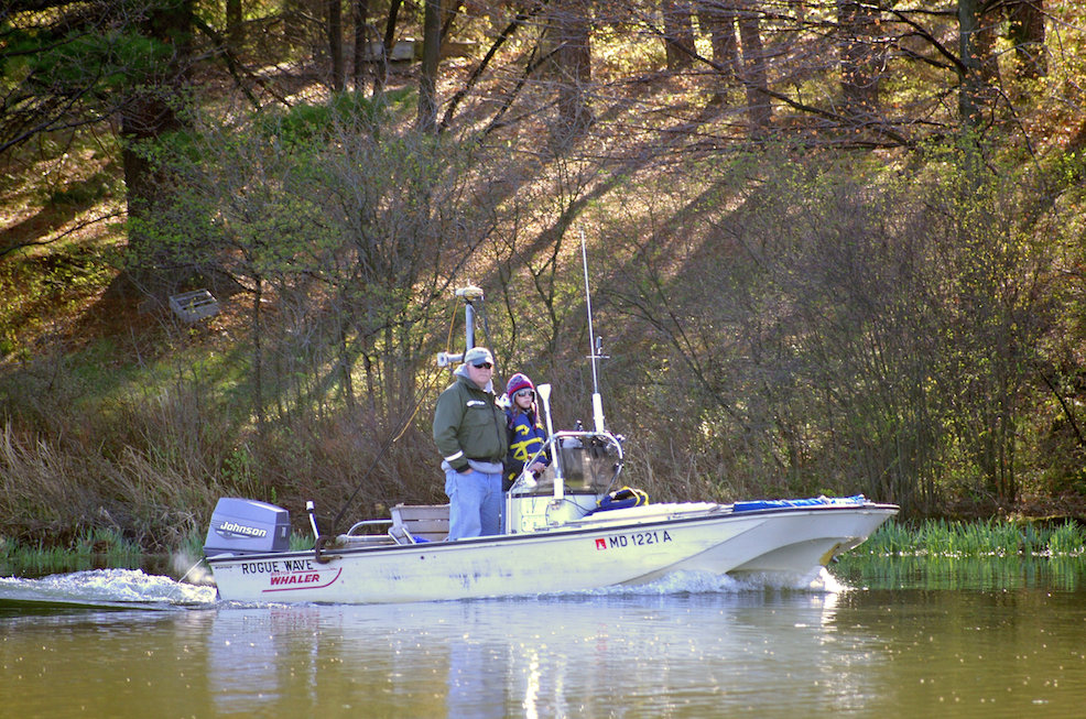
Figure 1. Richard Ortt and his Assistant taking Bathymetry Measurements of Deep Creek Lake.
We did some sanity checks with the data with Excel and after several email exchanges we discarded several hundred data records that were clearly bad, a very small amount considering.
I decided that the “R” language was to be learned for its graphics features and computational capability in order to process and display the various kinds of data. This turned out to be a major commitment, lasting four months to get to the ability to produce the graphs that are on this website. R has a very steep learning curve, but is very powerful and quite flexible.
The was time well spent.
Measurements were made on April 12 and 13, April 16 and 17 and April 19 through 21, all of 2012. This data set is the most recent one of the bathymetry of Deep Creek Lake. The original data were made available in Excel files and are contained in a zip file, here. DNR processed the raw data and produced a set of 6 files of true data.
NOTE: The following table provides a summary of the content of these 6 files. (Note: all subsequent tables created by taking a comma delimited file, such as produced with Excel, and submitting this to the following website:) The total number of data points are 617,419.
| Date | File Name | # of points | Min Lon | Max Lon | Min lat | Mx Lat | Min Depth | Max Depth |
|---|---|---|---|---|---|---|---|---|
| 12-Apr | April12xyz.txt | 48,445 | -79.32150017 | -79.25799367 | 39.484192 | 39.50689817 | 2.61 | 45.75 |
| 13-Apr | April13xyz.txt | 62,194 | -79.31166183 | -79.275382 | 39.492046 | 39.51567983 | 2.61 | 51.85 |
| 16-Apr | April16xyz.txt | 106,138 | -79.3207975 | -79.2765555 | 39.448169 | 39.49623683 | 2.51 | 46.73 |
| 17-Apr | April17xyz.txt | 116,506 | -79.32140633 | -79.24972417 | 39.46307867 | 39.5068495 | 2.54 | 36.65 |
| 19-Apr | April19xyz.txt | 90,057 | -79.34453133 | -79.28951433 | 39.46386267 | 39.53688867 | 2.51 | 59.28 |
| 20-Apr | April20xyz.txt | 97,236 | -79.39220833 | 39.55918633 | 39.44820533 | 39.55918633 | 3.49 | 59.61 |
| 21-Apr | April21xyz.txt | 96,843 | -79.39202017 | -79.344315 | 39.49837067 | 39.53027483 | 3.82 | 75.85 |
The first thing one does is to plot the data to see what it looks like. What became obvious early on in the work that the number of measurements made were far in excess of what would be useful. The distance between two data points along the path the boat was traveling was much, much smaller that the distance between two paths that the data-collecting boat took. This can be made to see with a simple R script in the following three plots.
{R pressure, echo=FALSE}
plot(pressure)
Along a path that the data-taking-boat When you click the Knit button a document will be generated that includes both content as well as the output of any embedded R code chunks within the document. You can embed an R code chunk like this:
{R cars}
summary(cars)
You can also embed plots, for example:
{R pressure, echo=FALSE}
plot(pressure)
Note that the echo = FALSE parameter was added to the code chunk to prevent printing of the R code that generated the plot.
To make the bathymetric maps and superimpose the boat slips on them required the following. The process how this was done is described in an other post on this blog.
To make the bathymetric maps and superimpose the boat slips on them required the following:
1. An outline of the the boundary of the lake. We obtained that from Debbie Carpenter, Garrett County Department of Planning and Zoning, in the form of an ESRI shape file.
2. A list of the locations of the boat slips. One of us digitized the boat slips (3,377) using Google Earth from an image dated 7/9/2011, the middle of the boating season. Google Earth turned out to be remarkably accurate.
3. Software (R has many “packages” to choose from; it was often not clear which one to go with) to process the irregularly spaced data points into regular data and from them create the depth contours and color coding system.
4. Conversion of data from lat/lon (as acquired by the gps system) to the Maryland State Plane Coordinate System because the lake outline was in those coordinates.
5. Write and test the software and produce the maps.
The following is a collection of preliminary maps that were produced using the over 600,000 measurements taken by Maryland’s Department of the Natural Resources in the spring (April) of 2012. The term ‘preliminary’ is used to designate that no suitable boundary, a boundary elevation at which the lake level depth was zero was available. It turns out that such suitable boundary at 2462 ft ASL was available, but only as a hard-drawn map but required its digitized, a process to cumbersome. This contour did surface later on in digitized form.
The maps that were subsequently developed with the “R” language for data processing and plotting and produced in different resolutions, 5ft, 10ft, 20ft, and 40 ft. They were also produced with different data interpolation methodologies. The maps that have been published here are the best of the batch, namely with the 10ft resolution and an interpolation method that provides results that appear to be good.
The coves and areas covered are shown in this overall map of Deep Creek Lake.
1. Anglers Cove
2. Arrowhead Cove
3. Blakeslee
4. Carmel Cove
5. Deep Creek Cove
6. Deep Creek Bridge
7. East Deep Creek Bridge
8. Glendale Bridge
9. Green Glade Cove
10. All of Green Glade
11. Harveys Cove
12. Hickory Ridge
13. High Mountain Sport
14. Hoop Pole
15. Lakeshore-1
16. Lakeshore-2
17. McHenry Coves
18. North Glade East
19. Pawn Run Cove
20. Penn Cove
21. Poland Run
22. South Center
23. South West
24. Sky Valley
25. Turkey Neck
26. Savage Cove
27. Glen Cove
28. Gravelly Run
29. Sandy Beach
30. Hazelhurst
Other maps:
* DNR’s 2012 Bathymetry Map of Deep Creek Lake (49.3 MB)
* USGS’s 2007-2008 Bathymetry Map of Deep Creek Lake (0.4 MB)
This is a list of links pointing towards the prime resources that were used to ultimately produce bathymetric maps.
1. The R language
2. Rstudio
PLV: First Published: 2012-12-16
Adapted for this website: 11/9/2017