Piet's Notes on Deep Creek Lake Science
Sensible Technologies - The Science of Deep Creek Lake
Here I have described how I generated the bathymetric maps of various coves of Deep Creek Lake using “R” and the data sets that have been created to make it work. I’ll show the steps I took, including code segments of important ideas, together with the resulting final maps. I’ll use Arrowhead Cove as an example since it is the target of possible dredging work. Detailed maps of the bathymetry of all of the coves are available on deepcreekanswers.com
In addition to these maps, I have created maps for all the coves that show when a typical boat on Deep Creek Lake becomes stranded if it were to remain in its boat slip. These will be made available on this website in the near future (today’s date is 9/5/2017; near is unspecified; a request would be encouraging)
Bathymetric maps of the coves of Deep Creek Lake can have a number of useful purposes. Among them are knowing how much water is under one’s boat at a given lake water level so that one can judge whether to move one’s boat slip further away from shore into deeper waters or remove the boat from the water entirely, finding the best fishing spots, determining how much dredging material to remove or assessing shore line erosion issues, and others.
The various mapping concepts are described here using Arrowhead Cove, because it is the principal candidate for removal of sediment by dredging.
The bathymetric work relies on several data sets that have been created separately and are discussed in a separate blog post.
These data sets are:
1. The raw measured bathymetric data points (collected by DNR in 2012)
2. The outline of the lake at the elevation of the spillway (2462 ft AMSL surveyed contour)
3. A rough set of coordinates defining that part of the lake for which the bathymetry is to be generated (digitized from a lake outline)
4. The coordinates of the boat slips (digitized from a GoogleMap image). For all 3,377 boat slips identifies check the file here
All of these data are taken at a point in time, but as one can guess, as time moves forward, their values change due to a number of natural and man-made effects. For example, one of most sought after data set, for me at least, was the 2462 ft AMSL surveyed contour because it provided ’the’ boundary condition for generating the lake’s bathymetry. That level changes with time due to erosion, landscaping and construction. These changes affect the boundary condition, but cannot be accounted for and may not be important. In the long run, a resurvey, or some other method, would be desired and then redo the bathymetry.
The image shown in Figure 1 is a typical result using the Akima interpolation method see Package ‘akima’ , and R_for_fun_learning or Google +R Akima interpolation of irregular spaced points.
Note the various elements on the plot, in addition to the bathymetry itself. In the upper left of the image is text that describes various aspects of the the method of generation, such as when it was plotted, the interpolation scheme used, the spatial resolution of the plot, and some geometry parameters.
On the lower left hand side is the color legend. Notice that the water levels in the depth contours are referenced to 2462 ft AMSL. In other words, when it says < 4 ft, that means that at a lake level of 2458 ft (2462-4), the land above this level is exposed land and not water. The third element is a small map of the whole lake and a circle identifying where this cove (Arrowhead) is located.
The Akima method, used for the map in Figure 1, for interpolating irregularly spaced data points, has been around for a long time and used successfully in many applications. An application by a third party is shown here.
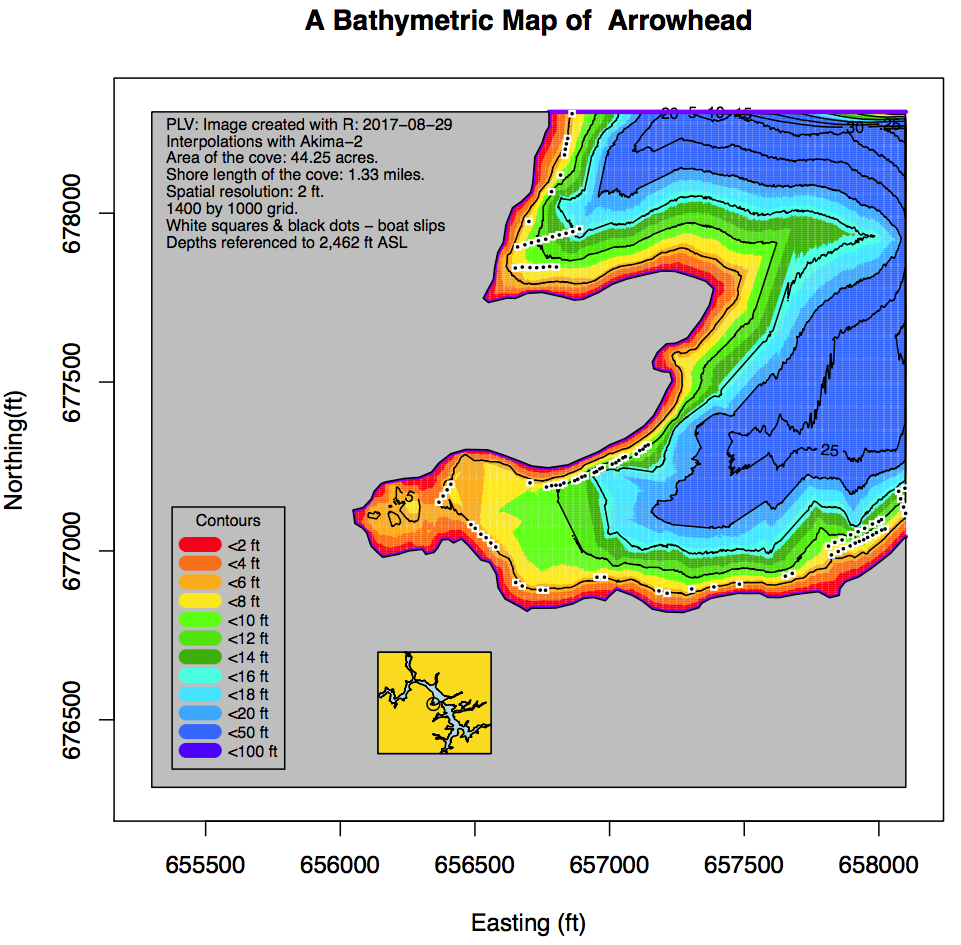
Figure 1. Akima Interpolation for Arrowhead Cove.
The next graph, Figure 2, is done with the MBA interpolation method.See the article: “Creating a DEM from regularly / irregularly spaced points (R and Python)” and Package ‘MBA’ The contours for the Arrowhead Cove are much smoother, more pleasing to the eye.
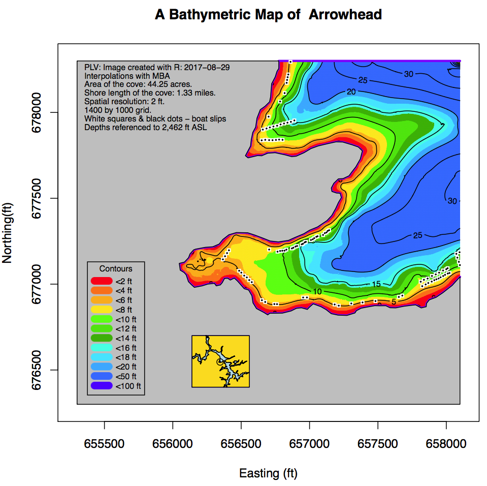
Figure 2. MBA Interpolation of Arrowhead Cove with 2ft Resolution.
In addition to these maps, a file is produced to contains the contours in Easting/Northing ft units for the first five contours. This data is for use by other software products, such as AutoCad. The first few feet are generally of interest so the data points for the first five contours are also written to a file. The following is the format of that file:
0	2
7396
dC.long	dC.lat	dC.piece
656089.556826305	677042.593716628	1
656090.495629399	677042.212716226	1
656091.024303074	677042.006752385	1
656092.491779843	677041.595465328	1
etc.
The data is in tab delimited format. Line 1: the range of the contour, here from 0 ft to 2 ft Line 2: The number of points on the contour (records; each line is a record) Line 3: Column headings. The ‘piece’ column is a sequential number indicating what piece of the contour the points belong to. The contour can be interrupted by a number of things. Line 4: (and following) the point coordinates in Easting and Northing ft and the ‘piece’ it belongs to. (I know, too many digits; this can be changed)
There are be five such sets in this file, as currently programmed, and only contours for the MBA method.
NOTE: One can change a lot of things: resolution, break points for the contour, number of significant digits, organization of the data (separate file for each contour?), comma separated, Akima, cove, etc. A sample data set can be found here.
To verify this data set it is plotted on a separate figure, Figure 3, which can be checked against the detailed figure above.
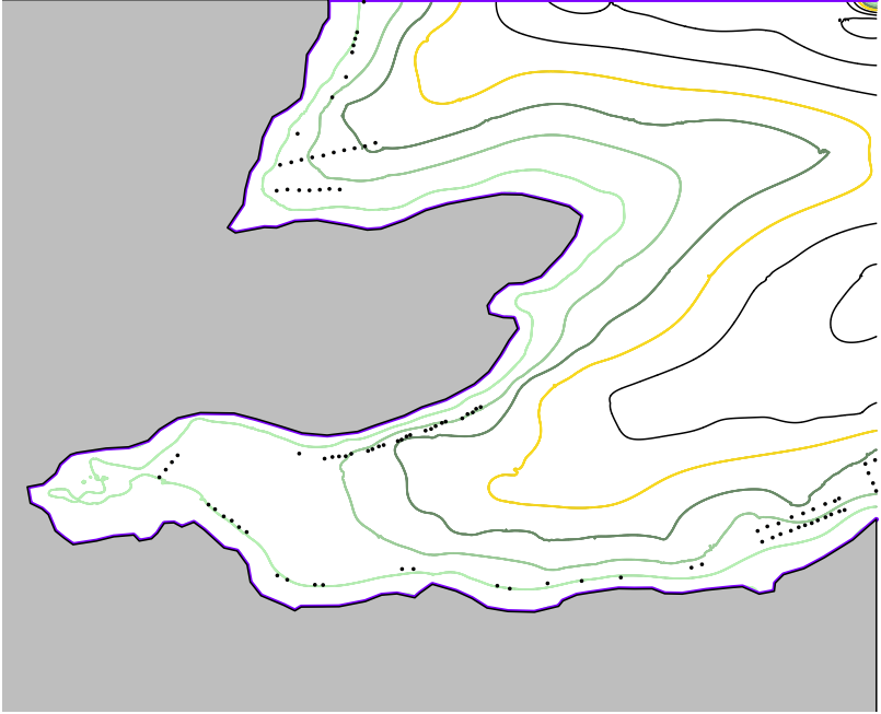
Figure 3. Arrowhead Extracted Contours.
One can create other maps that may be useful or instructive. First one can look at the amount of lake bottom that becomes exposed as the lake level drops. Probably the simplest way is to generate contours at one feet increments over a typical span of interest. Figure 4 is an example.
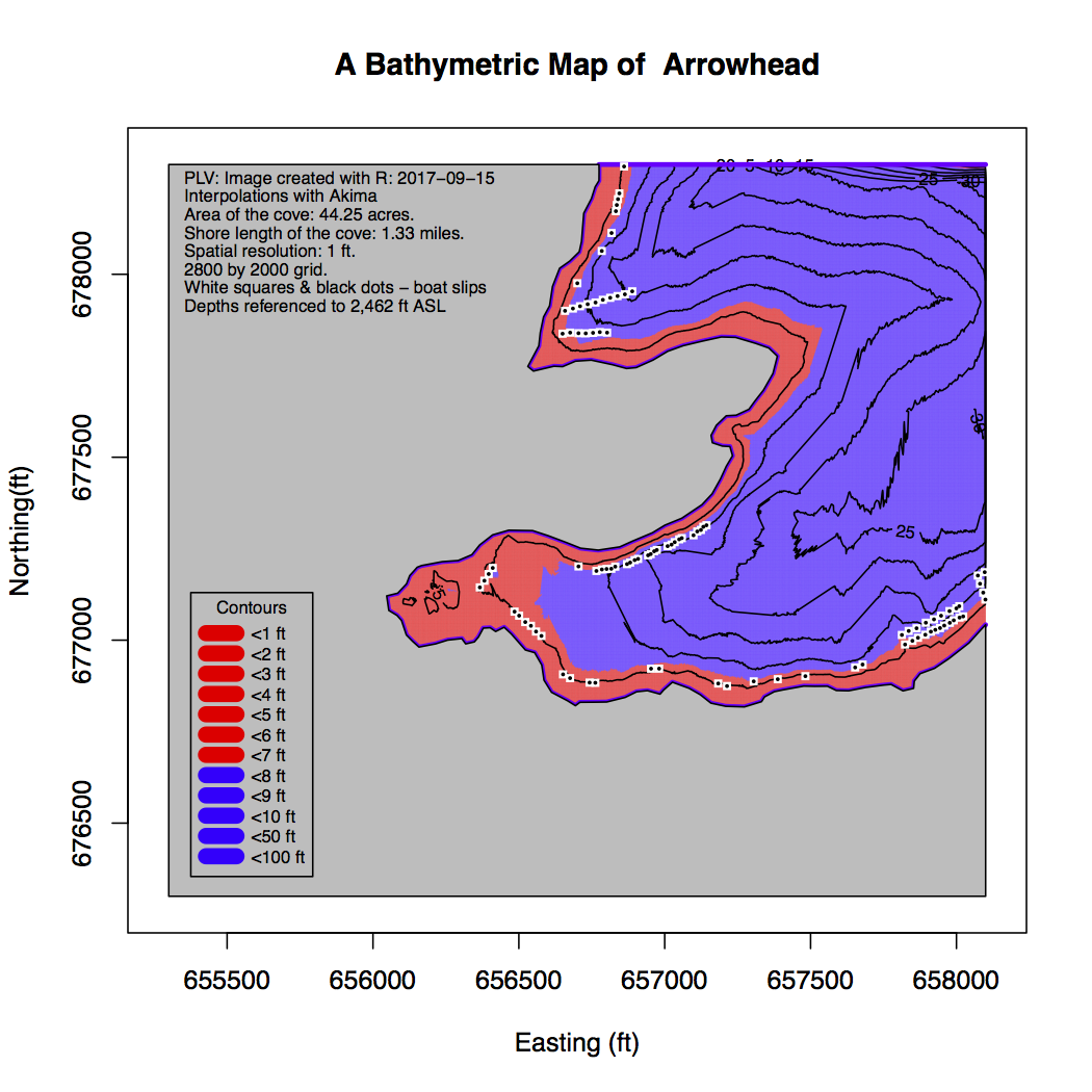
Figure 4. Arrowhead Mapping to Define Exposed Boat Slips.
To determine the span of interest one must understand the draft of a boat. For a typical popular brand boat seen around the lake, a Cobalt, the maximum draft with the drive down is listed as 37-inches.. To avoid cutting into the bottom, and perhaps hit a rock or two, and the action of waves and the add-on weight of the ‘helmsman’ and gear, a total comfortable minimum depth of water required is probably 4ft, or 48-inches. There are shallower draft boats, such as the family of different pontoon boats, but the location of a boat slip should probably be determined on the basis of the typical deepest draft boat, probably a Cobalt.
The maximum value of the current Lower Rule Band (LRB) is during the summer, from June 1 to July 1 at 2460 ft. The LRB falls from 2460 ft, at the beginning of July, to 2455 ft, at the beginning of December. The time span of interest is probably from July 1 to August 31, when the LRB drops from 2460 ft to 2458 ft.